Fit Transients

This guide shows how to model a series of multi-epoch images containing a transient.

import astropy.io.fits as fits
# Import Packages and setup
import jax.numpy as jnp
import matplotlib.pyplot as plt
from astropy.coordinates import SkyCoord
from astropy.wcs import WCS

import scarlet2 as sc2

sc2.set_validation(False)

We will load four ZTF images, in g and r band, from before and after the appearance of the transient. To speed up the processing and fitting, we have already resampled all images and PSFs to the same wcs using swarp, so we can create one Observation to hold all four images:

from huggingface_hub import hf_hub_download

filename = hf_hub_download(
    repo_id="astro-data-lab/scarlet-test-data",
    filename="transient_tutorial/data.fits.gz",
    repo_type="dataset",
)

data = []
weight = []
psf = []
channels = []
with fits.open(filename) as hdul:
    for i in range(4):
        # getting observation, weights, and PFS for each epoch
        idx = i * 3
        header = hdul[idx].header
        print("loading", header["FILENAME"])
        if i == 0:
            wcs = WCS(header)
        data.append(hdul[idx].data)
        weight.append(hdul[idx + 1].data)
        psf.append(hdul[idx + 2].data)

        # channel: combined band and epoch identifier
        # any labels is valid for each, e.g. timestamps
        channels.append((header["FILTER"], i))

obs = sc2.Observation(
    data,
    weights=weight,
    psf=psf,
    wcs=wcs,
    channels=channels,
    name="ZTF"
)

Warning: You are sending unauthenticated requests to the HF Hub. Please set a HF_TOKEN to enable higher rate limits and faster downloads.

loading ztf_20210519347083_000719_zg
loading ztf_20210519321944_000719_zr
loading ztf_20210705257257_000719_zg
loading ztf_20210731241088_000719_zr

Note

The channel attribute of the frame can be extended to identify different bands and epochs.

If we want to avoid the preprocessing step to resample and align the images (and PSFs), one can treat each image as its own Observation and resampling them on-the-fly (see the multi-resolution tutorial for details), but that makes the fitting much more computationally demanding.

But let’s look at what we have:

norm = sc2.plot.AsinhAutomaticNorm(obs)
sc2.plot.observation(obs, norm=norm, add_labels=False, show_psf=True);

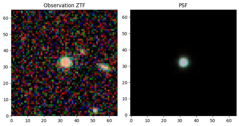
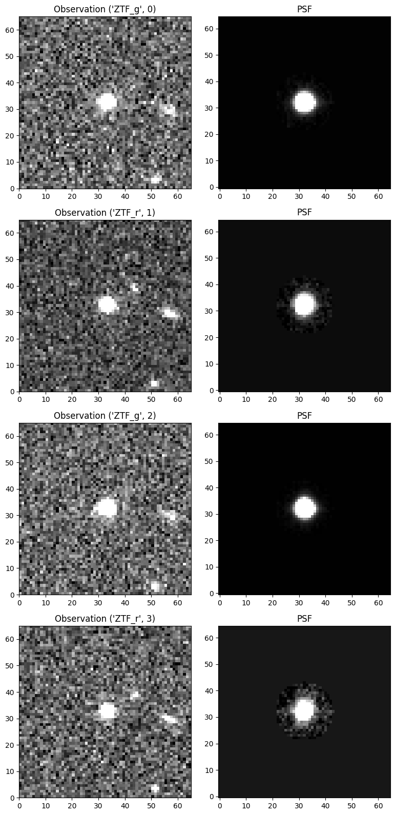
This is very much a false-color image because each channel (here there are four) is interpreted as a distinct band, but we actually only have g and r-bands. Because our plotting routines assumes channels are ordered with increasing wavelength, and the transient appears in the two latter epochs ,it’s visible as an excess in red in the color image above, slightly to the left of the source center. To see the channels separately, use the split_channels option for scarlet2.plot.observation():

sc2.plot.observation(obs, add_labels=False, show_psf=True, split_channels=True);

Define Transient Scene

We first need to define a model frame, which covers the same sky area as the data. As the ZTF PSF is not well-sampled, we reduce the internal model PSF to a very narrow Gaussian:

model_psf = sc2.GaussianPSF(sigma=0.5)
model_frame = sc2.Frame.from_observations(obs, model_psf=model_psf)

In scarlet2 we treat transients as sources that have independent amplitudes in every band and epoch (defined by TransientArraySpectrum), while static sources only have independent amplitudes in every band, i.e. their spectrum are shared across all epochs (implemented in StaticArraySpectrum). If we know that the transient is “off” for some epochs (e.g. pre-explosion), we can set those amplitudes to zero.

As our model frame treats the channels as a combined (band, epoch) identifier, the spectrum attributes for every source inherit this overloaded definition. So, we need to take care to set/fit the elements of this generalized spectrum vector correctly. For that purpose, we define lookup functions (band_selector and epoch_selector), which operate on the channel information and return the band or the epoch, respectively.

We can now define a Scene:

# coordinates of the transient
ra = 215.39425925333
dec = 37.90971372
coord = SkyCoord(ra, dec, unit="deg")

# separate channel information into band and epoch: 0 and 1 element
# depends on how channels encodes multi-epoch information
band_selector = lambda channel: channel[0]
epoch_selector = lambda channel: channel[1]

with sc2.Scene(model_frame) as scene:
    # 1) Host galaxy that is static across epochs
    try:
        spectrum, morph = sc2.init.from_gaussian_moments(obs, coord, box_sizes=[15, 21])
    except IndexError:
        morph = sc2.init.compact_morphology()
    # the host is barely resolved and the data are noisy:
    # use a parametric morphology for extra stability (esp to noise)
    n, size, ellipticity = 1., 2., jnp.zeros(2)
    morph = sc2.SersicMorphology(n, size, ellipticity, shape=morph.shape)

    # Select the transient-free epochs to initialize amplitudes for the static source
    # These will be shared across all epochs
    spectrum = spectrum[0:2]
    bands = ["ZTF_g", "ZTF_r"]
    sc2.Source(
        coord, sc2.StaticArraySpectrum(spectrum, bands=bands, band_selector=band_selector), morph
    )

    # 2) Point source for the transient, placed initially at same center
    # Define the epochs where the transient is allowed to have a non-zero amplitude
    epochs = [2, 3]
    # As we already know that the transient is present, we can measure the flux at the center location
    # This will be a mixture of host and transient light, to be corrected by the fitting procedure
    # Initializing as zero also works
    spectrum = sc2.init.pixel_spectrum(obs, coord)
    sc2.PointSource(
        coord, sc2.TransientArraySpectrum(spectrum, epochs=epochs, epoch_selector=epoch_selector)
    )

print(scene.sources)

[Source(
  center=f32[2],
  spectrum=StaticArraySpectrum(data=f32[2], bands=['ZTF_g', 'ZTF_r']),
  morphology=SersicMorphology(size=2.0, ellipticity=f32[2], n=1.0),
  bbox=Box(shape=(4, 15, 15), origin=(0, 25, 25)),
  components=[],
  component_ops=[]
), PointSource(
  center=f32[2],
  spectrum=TransientArraySpectrum(data=f32[4], epochs=[2, 3]),
  morphology=GaussianMorphology(size=0.5, ellipticity=None),
  bbox=Box(shape=(4, 9, 9), origin=(0, 28, 28)),
  components=[],
  component_ops=[]
)]

Fitting

Fitting works as usual by defining the Parameters. Because the two spectra and the host morphology (of type SersicMorphology) aren’t simple arrays but models themselves, their free parameters are the array attributes .data and the Sersic profile parameters, respectively, as show in the source definition above, e.g. TransientArraySpectrum(data=f32[4],...). These fundamental degrees of freedom of the scene is what we have to pass to the parameters class:

from numpyro.distributions import constraints

pos_step = 1e-2
SED_step = lambda p: sc2.relative_step(p, factor=5e-2)

with sc2.Parameters(scene):
    # Static host galaxy parameters
    sc2.Parameter(
        scene.sources[0].spectrum.data,
        name="spectrum_0",
        constraint=constraints.positive,
        stepsize=SED_step,
    )
    sc2.Parameter(
        scene.sources[0].center,
        name="center_0",
        stepsize=pos_step,
    )
    sc2.Parameter(
        scene.sources[0].morphology.n,
        name="n_0",
        constraint=constraints.interval(0.5, 4),
        stepsize=0.1,
    )
    sc2.Parameter(
        scene.sources[0].morphology.size,
        name="size_0",
        constraint=constraints.positive,
        stepsize=0.1,
    )
    sc2.Parameter(
        scene.sources[0].morphology.ellipticity,
        name="eps_0",
        constraint=sc2.constraint.unit_disk,  # enforces |e| < 1
        stepsize=1e-2,
    )

    # Transient point source parameters:
    # no positive constraint on spectrum because it can be zero
    sc2.Parameter(scene.sources[1].spectrum.data, name="spectrum_1", stepsize=SED_step)
    sc2.Parameter(
        scene.sources[1].center, name="center_1", constraint=constraints.positive, stepsize=pos_step
    )

# Fit the scene
stepnum = 1000
scene_ = scene.fit(obs, max_iter=stepnum, e_rel=1e-4)

Inspect Result

# Plot the model, for each epoch
sc2.plot.scene(
    scene_,
    observation=obs,
    norm=norm,
    show_model=True,
    show_observed=True,
    show_rendered=True,
    show_residual=True,
    add_labels=True,
    add_boxes=True,
    split_channels=False,
    box_kwargs={"edgecolor": "red", "facecolor": "none"},
    label_kwargs={"color": "red"},
)
plt.show()

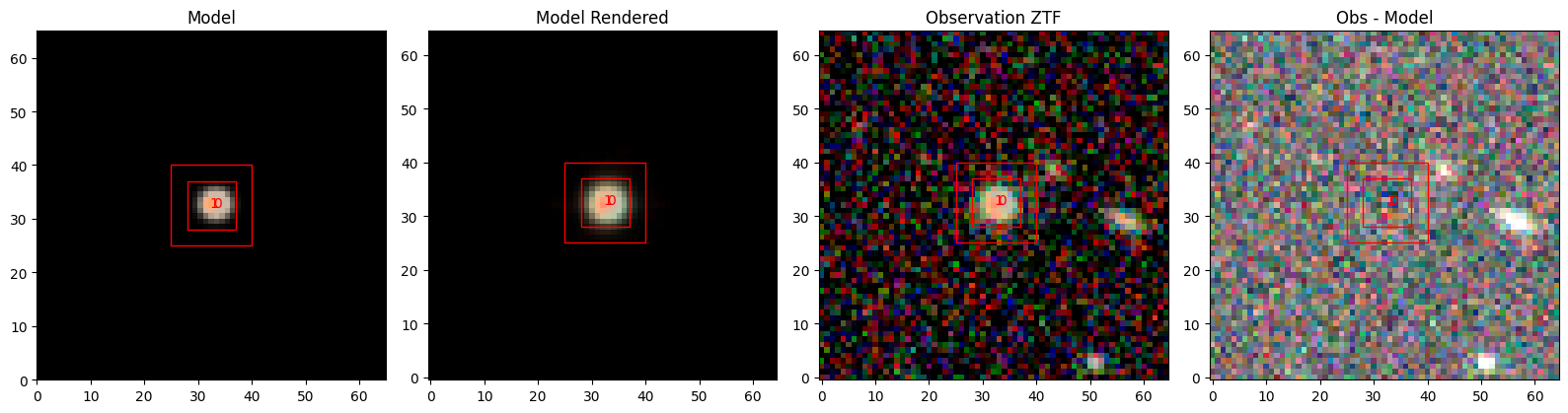
Looks good, modest reddening on the left of the center, with no noticeable residuals. Here are the best-fitting fluxes:

print("----------------- {}".format(channels))
for k, src in enumerate(scene_.sources):
    print("Source {}, Fluxes: {}".format(k, sc2.measure.flux(src)))

----------------- [('ZTF_g', 0), ('ZTF_r', 1), ('ZTF_g', 2), ('ZTF_r', 3)]
Source 0, Fluxes: [2182.804  3128.1594 2182.804  3128.1594]
Source 1, Fluxes: [   0.         0.       654.31757 1160.6621 ]

Note that the host galaxy, source 0, has the same flux in each epoch of the same band, while the transient, source 1, has zero flux in the epochs where we forced it to be ‘off’.