Quick Start Guide#
This notebook walks through the scarlet2 workflow to model and deblend two synthetic Gaussian sources with different colors, just to see the basic functionality.
from functools import partial

import jax
import jax.numpy as jnp
import matplotlib.pyplot as plt
from numpyro.distributions import constraints

import scarlet2 as sc2
Generate Synthetic Data#
We create a 3-band image with two overlapping Gaussian sources. The channels are ordered from short to long wavelength, we’ll call them (b, g, r).
Source 1 (center pixel 20, 20) is bright in the red band.
Source 2 (center pixel 30, 28) is bright in the blue band.
shape = (51, 51)
channels = ["b", "g", "r"]
noise_sigma = 0.2

# True source parameters (y, x convention)
centers = [jnp.array([20.0, 20.0]), jnp.array([30.0, 28.0])]
sigmas = [4.0, 6.0]
true_spectra = [
    jnp.array([1.0, 3.0, 10.0]),  # red source: faint in b, bright in r
    jnp.array([10.0, 3.0, 1.0]),  # blue source: bright in b, faint in r
]

# Build data cube: sum of two unnormalized 2D Gaussians
y, x = jnp.mgrid[:shape[0], :shape[1]]
data = jnp.zeros((len(channels), *shape))
for center, sigma, spectrum in zip(centers, sigmas, true_spectra):
    r2 = (y - center[0]) ** 2 + (x - center[1]) ** 2
    morph = jnp.exp(-r2 / (2 * sigma ** 2))
    data = data + spectrum[:, None, None] * morph[None]

# Add Gaussian noise
key = jax.random.key(42)
noise = jax.random.normal(key, data.shape) * noise_sigma
data = data + noise
weights = jnp.full(data.shape, 1 / noise_sigma ** 2)
Create the Observation#
An Observation packages the data and the weights and a description of the piece of sky we want to describe. We call the latter a Frame, which stores additional information, such channel labels and PSF model (which we don’t use here).
obs = sc2.Observation(
    data,
    weights=weights,
    channels=channels,
)
Observation validation results:
[000]   INFO    Number of channels in the observation matches the data.
[001]   INFO    Data and weights have the same shape.
[002]   INFO    Observation.weights in the observation are finite and non-negative.
[003]   INFO    Data in the observation are finite where weights are greater than zero.
[004]   WARN    Observation.psf is not defined.
Note the validation results, which are automatically generated (unless switched off) and act as early warning signs. For additional information about automatic validation, check out the Validation guide.
The observation metadata are now stored in obs.frame:
print(obs.frame)
Frame(
  bbox=Box(shape=(3, 51, 51), origin=(0, 0, 0)),
  psf=None,
  wcs=WCS Keywords

      Number of WCS axes: 2
      CTYPE : 'RA---TAN' 'DEC--TAN'
      CRVAL : np.float64(0.0) np.float64(0.0)
      CRPIX : np.float64(26.0) np.float64(26.0)
      PC1_1 PC1_2  : np.float64(1.0) np.float64(0.0)
      PC2_1 PC2_2  : np.float64(0.0) np.float64(1.0)
      CDELT : np.float64(1.0) np.float64(1.0)
      NAXIS : 51  51,
  channels=['b', 'g', 'r']
)
As you can see, the frame contains the size of the data array, WCS information on what area of the sky is being described (it’s trivial here: RA/DEC = 0,0), and the description of the channels in the observation.
In scarlet2, we use the term “channel” for any dimension that is not in the plane of the sky. It could be photometric bands (like the three bands in this example), spectroscopic wavelengths, and/or time. I’s the third axis of the image cube.
Display the Image Cube#
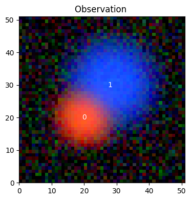
We can now plot the observation as a RGB image with a brightness scaling that shows both the brightest parts and the noise floor:
norm = sc2.plot.AsinhAutomaticNorm(obs)
sc2.plot.observation(obs, norm=norm, sky_coords=jnp.stack(centers), add_labels=True)
plt.show()
Define the Model Frame#
We want to model the sky using the observation we have, and for that we need to define the properties of the model. That is, we need a Frame from our model. In this very simple example, we can make it identical to the data frame:
model_frame = obs.frame
In general, we’ll want to define the model frame differently, e.g. giving it a constant PSF to account for PSF variations across the observation bands (as in our real-world example), or extending the portion of the sky we model to accommodate multiple slightly offset observation (as in our multi-observation tutorial).
Initialize Sources#
We can now construct a Scene using a with block. Any Source created inside that block is automatically added to the scene. This is the model of the sky we want to build and then optimize.
Each source needs a center, a spectrum (1D, one value per channel), and a morphology (2D, one value for each pixel of the model frame). The source combines these into a model of the data cube by the outer product spectrum x morphology. scarlet2 implements several different spectrum and morphology models (e.g. SersicMorphology), but the simplest approach is to use ordinary 1D and 2D arrays, so that every element is a free parameter of the model (a so-called “non-parametric” model).
Tip
scarlet2 can mix parametric and non-parametric models as you see fit. It is also easy to extend when you need a model we don’t already provide.
We could initialize spectrum and morphology as random or even zero-valued arrays. But it’s better to get an initial guess that is closer to the desired solution, so we use the method from_gaussian_moments() to initialize these arrays. The method measures the moments of the brightness distribution in the data at each center, reports the 0th moments across the channels as the 1D array spectrum, and creates a 2D Gaussian image morph from the 2nd moments:
with sc2.Scene(model_frame) as scene:
    for center in centers:
        spectrum, morph = sc2.init.from_gaussian_moments(obs, center, box_sizes=[31, ])
        sc2.Source(center, spectrum, morph)

print(scene)
Scene(
  frame=Frame(
    bbox=Box(shape=(3, 51, 51), origin=(0, 0, 0)),
    psf=None,
    wcs=WCS Keywords

        Number of WCS axes: 2
        CTYPE : 'RA---TAN' 'DEC--TAN'
        CRVAL : np.float64(0.0) np.float64(0.0)
        CRPIX : np.float64(26.0) np.float64(26.0)
        PC1_1 PC1_2  : np.float64(1.0) np.float64(0.0)
        PC2_1 PC2_2  : np.float64(0.0) np.float64(1.0)
        CDELT : np.float64(1.0) np.float64(1.0)
        NAXIS : 51  51,
    channels=['b', 'g', 'r']
  ),
  sources=[
    Source(
      center=f32[2],
      spectrum=f32[3],
      morphology=f32[31,31],
      bbox=Box(shape=(3, 31, 31), origin=(0, 5, 5)),
      components=[],
      component_ops=[]
    ),
    Source(
      center=f32[2],
      spectrum=f32[3],
      morphology=f32[31,31],
      bbox=Box(shape=(3, 31, 31), origin=(0, 15, 13)),
      components=[],
      component_ops=[]
    )
  ]
)
scene contains the frame and the list sources. Each source has three data portions, indicating their shapes, e.g., f32[31,31], which denotes an 32 bit floating point array of 31x31 pixels. Let’s look at them:
sc2.plot.scene(
    scene, obs, norm=norm,
    show_model=True, show_observed=True, show_residual=True,
    add_boxes=True,
)
plt.show()
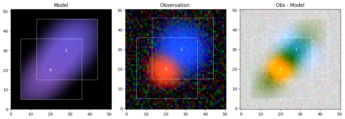
Well, that’s quite terrible… But that happens when we try to perform measurements (like the moments for the initialization method) on sources that are “blended”, meaning they are too close together: The properties we’d like to measure are mixed up.
Fit the Model#
We will now optimize the model. And for that we need to mark which model parameters should be updated by the optimizer. We define a collection Parameters of the model scene. Each Parameter created inside the with block needs to point to a data portion of the scene and give it a name, a stepsize, and an optional constraint. Here we use the following:
Spectra must be positive.
Morphologies are treated as pixel arrays constrained to the unit interval
[0, 1].
The purpose of these constraints is to reduce the number of options for the model parameters and thus the degeneracies that arise for complex models, especially of blended sources. As we think of celestial sources as emitters (not absorbers) of photons, it is reasonable to enforce that their models be positive. The unit constraint for the morphologies ensures that the brightness of the sources is adjusted only through spectrum.
spec_step = partial(sc2.relative_step, factor=0.1)
morph_step = partial(sc2.relative_step, factor=0.001)

with sc2.Parameters(scene):
    for i in range(len(scene.sources)):
        sc2.Parameter(
            scene.sources[i].spectrum,
            name=f"spectrum:{i}",
            constraint=constraints.positive,
            stepsize=spec_step,
        )
        sc2.Parameter(
            scene.sources[i].morphology,
            name=f"morph:{i}",
            constraint=constraints.unit_interval,
            stepsize=morph_step,
        )
We can now run the fitting method. We use optax.adam as the optimizer, which will employ the parameter-specific stepsizes as defined above.
scene_ = scene.fit(obs, max_iter=1000, e_rel=1e-4)
Running validation checks on the fit of the scene for observation .
Fit validation results:
[000]   INFO    The model fit is good. | Context={'chi2': Array(0.77330565, dtype=float32)})
[001]   INFO    The chi-square in the box for source 0 is good. | Context={'chi2_in': Array(0.58051777, dtype=float32), 'source': 0})
[002]   INFO    The chi-square in the border for source 0 is good. | Context={'chi2_border': Array(0.86368316, dtype=float32), 'source': 0})
[003]   INFO    The chi-square in the box for source 1 is good. | Context={'chi2_in': Array(0.53218573, dtype=float32), 'source': 1})
[004]   INFO    The chi-square in the border for source 1 is good. | Context={'chi2_border': Array(0.99520385, dtype=float32), 'source': 1})
The optimizer minimizes the loss function, which for every principled probabilistic model is given by the negative log-likehood of the model given the data.
Inspect Results#
The validations already ran, and it all looks good. Let’s check out the updated model scene_:
sc2.plot.scene(
    scene_, obs, norm=norm,
    show_model=True, show_observed=True, show_residual=True,
    add_boxes=True,
)
plt.show()
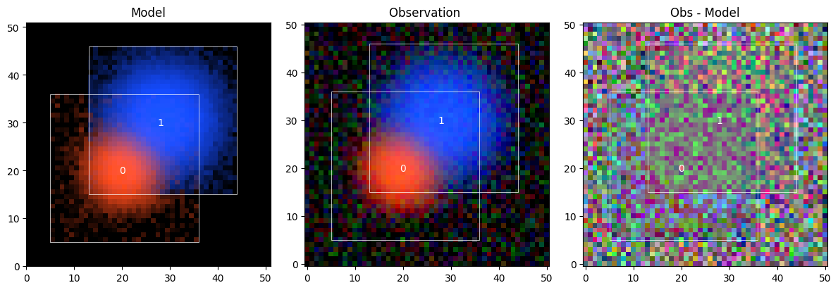
This is much better than before. The fitter used the difference in color to separate, aka deblend, the two sources. But the outskirts of the source models look noisy. We can plot the sources individually to get a better sense of it:
sc2.plot.sources(scene_, obs, norm=norm, show_observed=True, add_boxes=True)
plt.show()
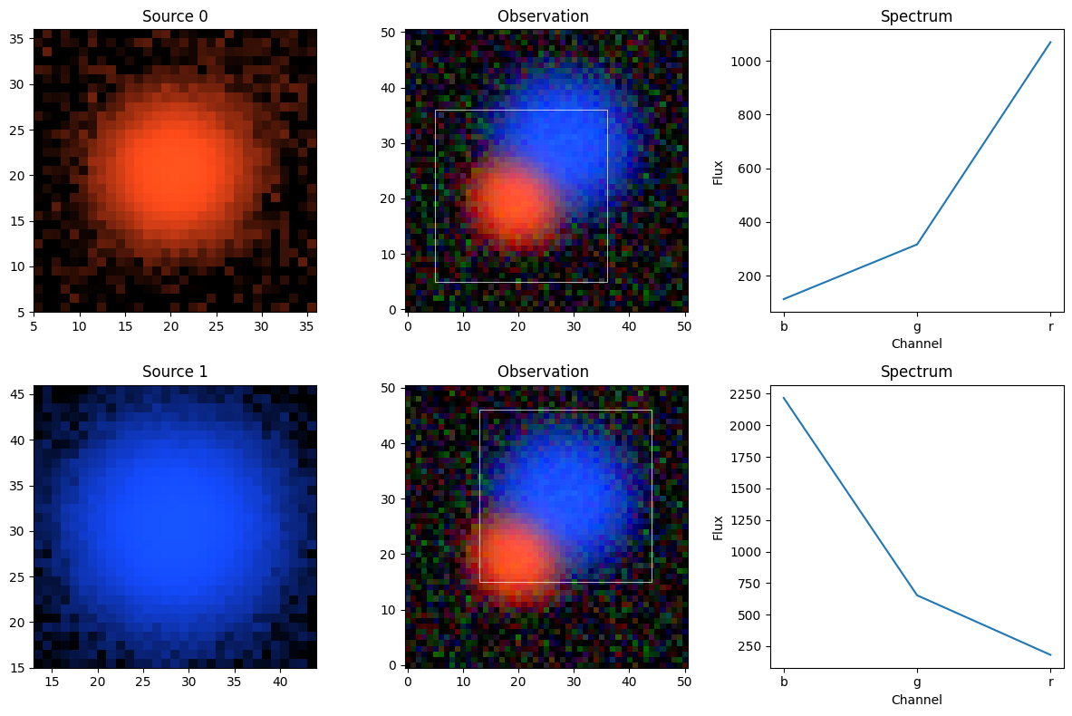
Because the models are non-parametric, every pixel and every spectrum channel can be adjusted separately, which means the optimizer will use this freedom to fit the data as best as possible, including the noise. While the spectrum is an integrated quantity and thus more robust to noise, the morphology arrays will often pick up noise.
We can evaluate the model by calling it: scene_() computes the model as a hyperspectral data cube over the entire model frame, from which we can determine the goodness of fit (defined as the average chi^2) of the model given the observation:
print(obs.goodness_of_fit(scene_()))
0.77330565
A good fit gives an average chi^2 close to 1 (one noise unit per pixel), which mean that our model overfits the data. Is that a big problem?
Source Measurements#
The per-band flux of each source is the integral of spectrum × morphology over the bounding box. Because we know that the sources are actually Gaussian, we can compute the true integrated fluxes as spectrum × 2π σ² and compare to our source models:
true_fluxes = [
    spectrum * 2 * jnp.pi * sigma ** 2
    for spectrum, sigma in zip(true_spectra, sigmas)
]

print(f"{'':12s}  {'b':>10s}  {'g':>10s}  {'r':>10s}")
for k, src in enumerate(scene_.sources):
    recovered = sc2.measure.flux(src)
    true = true_fluxes[k]
    print(f"Source {k} true:    {true[0]:10.2f}  {true[1]:10.2f}  {true[2]:10.2f}")
    print(f"Source {k} modeled: {recovered[0]:10.2f}  {recovered[1]:10.2f}  {recovered[2]:10.2f}")
                       b           g           r
Source 0 true:        100.53      301.59     1005.31
Source 0 modeled:     112.33      316.01     1069.22
Source 1 true:       2261.95      678.58      226.19
Source 1 modeled:    2217.27      653.21      181.13
Not perfect, but close. We can see that source 0 “steals” a bit of light from source 1, and, as we saw above, both are somewhat affected by noise. In other tutorials we will see how to manage these tendencies, either by using more restrictive parametric models or neural network priors. But this example demonstrates that even with no model assumptions and minimal constraints, the data alone are already highly informative. We just needed a properly specified model, the likelihood optimization did the rest.