Real-World Example#
This guide shows you how to model a scene from HyperSuprimeCam (HSC) data as a hyperspectral image cube.
# Import Packages and setup
import jax.numpy as jnp
import matplotlib.pyplot as plt

import scarlet2 as sc2
Load the Data#
We load the example data set (here an image cube from HSC with 5 bands) and a detection catalog. If such a catalog is not available, packages like SEP and photutils will happily generate one.
To make tests like this one convenient, we provide a HuggingFace data set for scarlet2. To download it locally, you need to pip install huggingface_hub:
from huggingface_hub import hf_hub_download

filename = hf_hub_download(
    repo_id="astro-data-lab/scarlet-test-data", filename="hsc_cosmos_35.npz", repo_type="dataset"
)
file = jnp.load(filename)
data = file["images"]
channels = [str(f) for f in file["filters"]]
centers = jnp.array([(src["y"], src["x"]) for src in file["catalog"]])  # Note: y/x convention!
weights = 1 / file["variance"]
psf = file["psfs"]
Warning: You are sending unauthenticated requests to the HF Hub. Please set a HF_TOKEN to enable higher rate limits and faster downloads.
Warning
Coordinates in scarlet are given in the C/numpy notation (y,x) as opposed to the more conventional (x,y) ordering.
Define the Observation#
An Observation stores several data arrays. In addition to the actual science image cube, you can and usually must provide weights for all elements in the data cube, an image cube of the PSF model (one image for each channel), an astropy.wcs.WCS structure to translate from pixel to sky coordinates, and labels for all channels.
The observation stores these meta-data in the data structure Frame as the attribute .frame (similar to the header in a FITS file).
obs = sc2.Observation(data, weights=weights, psf=psf, channels=channels)
Observation validation results:
[000]   INFO    Number of channels in the observation matches the data.
[001]   INFO    Data and weights have the same shape.
[002]   INFO    Observation.weights in the observation are finite and non-negative.
[003]   INFO    Data in the observation are finite where weights are greater than zero.
[004]   INFO    PSF is 3-dimensional.
[005]   INFO    Number of PSF channels matches the number of data channels.
[006]   WARN    PSF centroid is not the same in all channels. | Context={'psf_centroid': array([[ 0.04197121, -0.01779556,  0.0002327 ,  0.04332542,  0.06899071],
       [ 0.09050751,  0.01180649, -0.03284836,  0.08525848, -0.00099373]],
      dtype=float32)})
Note the validation results, which are automatically generated and act as early warning signs.
We’ll see more of these validation tests later in this notebook.
Here the check number 006 indicates that the PSF is not centered at the same position for all channels.
The offsets are minor, so we’ll proceed, but we’re going to come back to this issue at the end.
For additional information about automatic validation (including how to switch them off), check out the “Validation” section of the documentation.
Display the Image Cube#
We can now make use of the plotting function scarlet2.plot.observation() to create a RGB image of our data.
We’re going to use the AsinhAutomaticNorm, which scales the observed data by a \(\mathrm{sinh}^{-1}\) function that is automatically tuned to reveal both the noise level and the highlights, to create a color-consistent RGB image.
norm = sc2.plot.AsinhAutomaticNorm(obs)
sc2.plot.observation(obs, norm=norm, sky_coords=centers, show_psf=True, add_labels=True)
plt.show()
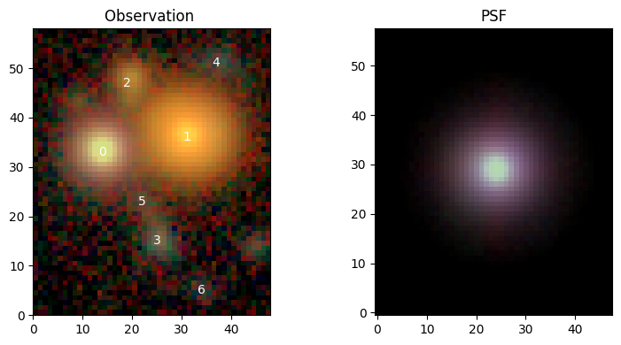
Since we did’t provide a wcs for this Observation, all spatial coordinates (like centers above) are in image pixels. Otherwise RA/Dec coordinates (as astropy.SkyCoord) are required.
Define the Model Frame#
scarlet2 needs another Frame, which describes the properties of the model of the sky you seek to fit. Given one or several observations, scarlet2 can make an educated guess what model frame would be best:
model_frame = sc2.Frame.from_observations(obs)
print(model_frame)
Frame(
  bbox=Box(shape=(5, 58, 48), origin=(0, 0, 0)),
  psf=GaussianPSF(morphology=GaussianMorphology(size=0.7, ellipticity=None)),
  wcs=WCS Keywords

      Number of WCS axes: 2
      CTYPE : 'RA---TAN' 'DEC--TAN'
      CRVAL : np.float64(0.0) np.float64(0.0)
      CRPIX : np.float64(25.0) np.float64(30.0)
      PC1_1 PC1_2  : np.float64(1.0) np.float64(0.0)
      PC2_1 PC2_2  : np.float64(0.0) np.float64(1.0)
      CDELT : np.float64(1.0) np.float64(1.0)
      NAXIS : 48  58,
  channels=['g', 'r', 'i', 'z', 'y']
)
If only one observation is given (as above), we assume that bands and pixel locations are identical between the model and the observation. Because we have ground-based images, we need to account for different PSFs in each band, which means the model frame needs to define a reference PSF that is sufficiently narrow. Our default is a minimal Gaussian PSF that is barely well-sampled (standard deviation of 0.7 pixels) as the PSF reference.
If other properties of the model frame are desired, they can be provided to scarlet2.Frame.from_observations().
But what’s the point of the model frame? Why is it needed at all?
Tip
To fit multiple images with different PSF, different bands, different resolutions, etc…, we must define a model that is superior in all of these aspects, so that each observation can be computed from the model by a degradation operation, the so-called “forward operator”. The point of joint modeling is to find one superior model of the sky that is consistent with all observations.
In scarlet2, the forward operators are implemented as Renderer, which contains, e.g., PSF difference kernels and resampling transformations. It gets created when calling ~scarlet2.Observation.match (which is normally done only when needed, but we can call it explicitly to see its effect):
obs.match(model_frame)
print(obs.renderer)
ConvolutionRenderer(kernel_fft=c64[5,96,33], shift=f32[2])
Initialize Sources#
You now need to define sources that are going to be fit. The full model, which we will call Scene, is a collection of Sources. Each source contains at least one Component, and each of those is defined by a center, spectrum, and morphology. You can have as many sources in a scene, or as many components in a source, as you want. To represent stars or other point sources, we provide the class PointSource, which adopts the PSF of the model frame as the morphological model of the source.
Adding sources to a scene is easy. You create the scene (as a python context with the with keyword) and then create a source inside of that context. It will automatically be added to the overall scene model. But now we have to decide what the initial values of spectrum and morphology should be. You can choose them as you see fit, but we also provide convenience methods. For instance scarlet2.init.pixel_spectrum() takes the spectrum of one pixel (typically the center pixel), and scarlet2.init.from_gaussian_moments() measures the spectrum and morphology by measuring the 2nd moments and creating an elliptical Gaussian to match those.
with sc2.Scene(model_frame) as scene:
    for center in centers:
        try:
            spectrum, morph = sc2.init.from_gaussian_moments(obs, center)
        except ValueError:
            # if the default init fails, fall back to
            # - spectrum from the center of the source
            # - morphology from the shape of a point source
            spectrum = sc2.init.pixel_spectrum(obs, center)
            morph = sc2.init.compact_morphology()

        sc2.Source(center, spectrum, morph)
If we know something about the scene, we might want to customize the modeling. Let’s assume that we know that object 0 is a star. We could just replace that source with a PointSource, but for clarity we rebuild the entire source list, making one change for source 0 and accepting everything else from the default initialization above:
with sc2.Scene(model_frame) as scene:
    for i, center in enumerate(centers):
        if i == 0:  # we know source 0 is a star
            spectrum = sc2.init.pixel_spectrum(obs, center, correct_psf=True)
            sc2.PointSource(center, spectrum)
        else:
            try:
                spectrum, morph = sc2.init.from_gaussian_moments(obs, center)
            except ValueError:
                spectrum = sc2.init.pixel_spectrum(obs, center)
                morph = sc2.init.compact_morphology()

            sc2.Source(center, spectrum, morph)
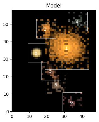
We can now check what we have in scene:
sc2.plot.scene(
    scene,
    obs,
    norm=norm,
    show_model=True,
    show_rendered=True,
    show_observed=True,
    show_residual=True,
    add_boxes=True,
);
print(scene)
Scene(
  frame=Frame(
    bbox=Box(shape=(5, 58, 48), origin=(0, 0, 0)),
    psf=GaussianPSF(morphology=GaussianMorphology(size=0.7, ellipticity=None)),
    wcs=WCS Keywords

        Number of WCS axes: 2
        CTYPE : 'RA---TAN' 'DEC--TAN'
        CRVAL : np.float64(0.0) np.float64(0.0)
        CRPIX : np.float64(25.0) np.float64(30.0)
        PC1_1 PC1_2  : np.float64(1.0) np.float64(0.0)
        PC2_1 PC2_2  : np.float64(0.0) np.float64(1.0)
        CDELT : np.float64(1.0) np.float64(1.0)
        NAXIS : 48  58,
    channels=['g', 'r', 'i', 'z', 'y']
  ),
  sources=[
    PointSource(
      center=f32[2],
      spectrum=f32[5],
      morphology=GaussianMorphology(size=0.7, ellipticity=None),
      bbox=Box(shape=(5, 11, 11), origin=(0, 28, 9)),
      components=[],
      component_ops=[]
    ),
    Source(
      center=f32[2],
      spectrum=f32[5],
      morphology=f32[25,25],
      bbox=Box(shape=(5, 25, 25), origin=(0, 24, 19)),
      components=[],
      component_ops=[]
    ),
    Source(
      center=f32[2],
      spectrum=f32[5],
      morphology=f32[11,11],
      bbox=Box(shape=(5, 11, 11), origin=(0, 42, 14)),
      components=[],
      component_ops=[]
    ),
    Source(
      center=f32[2],
      spectrum=f32[5],
      morphology=f32[11,11],
      bbox=Box(shape=(5, 11, 11), origin=(0, 10, 20)),
      components=[],
      component_ops=[]
    ),
    Source(
      center=f32[2],
      spectrum=f32[5],
      morphology=f32[11,11],
      bbox=Box(shape=(5, 11, 11), origin=(0, 46, 32)),
      components=[],
      component_ops=[]
    ),
    Source(
      center=f32[2],
      spectrum=f32[5],
      morphology=f32[11,11],
      bbox=Box(shape=(5, 11, 11), origin=(0, 18, 17)),
      components=[],
      component_ops=[]
    ),
    Source(
      center=f32[2],
      spectrum=f32[5],
      morphology=f32[11,11],
      bbox=Box(shape=(5, 11, 11), origin=(0, 0, 29)),
      components=[],
      component_ops=[]
    )
  ]
)
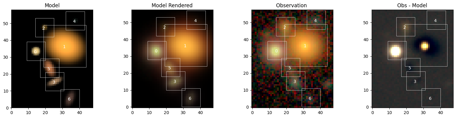
scene contains the frame and the list sources. The first source is a PointSource, which has a morphology model, namely the same GaussianMorphology as the PSF of the model frame.
All others are standard Sources. The data portions in these models are listed as, e.g., f32[11,11], which denotes an image array of 11x11 pixels. The size of these boxes was determined by scarlet2.init.from_gaussian_moments() to contain most of the flux (or the largest box that seems to be occupied by only one source).
But these initial choices are not great. So, we now have to…
Fit the Model#
The Scene class holds the list of sources and creates a model of the sky that (like any Module) can be evaluated, which allows us to determine the log-likelihood of the data given the model:
scene_array = scene()  # evaluate the model
print("Initial likelihood:", obs.log_likelihood(scene_array))
Initial likelihood: -3029193.5
But as most of us don’t think in terms of likelihoods, we can also compute the goodness of fit of the model, which is identical to the log-likelihood up to a constant but much easier to interpret: It’s the average chi^2 over all pixels with non-zero weights.
print("Avg. chi^2:", obs.goodness_of_fit(scene_array))
Avg. chi^2: 433.39108
You can now write your own fitter or sampler, but we provide the machinery for that as well. We’re using optax for the optimization. First we need to define which Parameters of the model should be optimized. A model parameter that is not included will not be updated. For each Parameter, you need to specify a name, stepsize, and, optionally, differentiable constraints or prior distributions from numpyro. Below is our recommended configuration:
from functools import partial
from numpyro.distributions import constraints

# best step size for parameters with a relative "uncertainty":
# big/bright sources adjust more quickly
spec_step = partial(sc2.relative_step, factor=0.05)
morph_step = partial(sc2.relative_step, factor=1e-3)

with sc2.Parameters(scene):
    for i in range(len(scene.sources)):
        sc2.Parameter(
            scene.sources[i].spectrum,
            name=f"spectrum:{i}",
            constraint=constraints.positive,
            stepsize=spec_step,
        )
        if i == 0:
            sc2.Parameter(scene.sources[i].center, name=f"center:{i}", stepsize=0.1)
        else:
            sc2.Parameter(
                scene.sources[i].morphology,
                name=f"morph:{i}",
                constraint=constraints.unit_interval,
                stepsize=morph_step,
            )
The parameters are now attached to scene, and can be accessed with scene.parameters.
Now we can run the fitting method:
maxiter = 1000
scene_ = scene.fit(obs, max_iter=maxiter, e_rel=1e-4)
Running validation checks on the fit of the scene for observation .
Fit validation results:
[000]   INFO    The model fit is good. | Context={'chi2': Array(1.315585, dtype=float32)})
[001]   WARN    The chi-square in the box for source 0 is acceptable, but not optimal. | Context={'chi2_in': Array(2.3210852, dtype=float32), 'source': 0})
[002]   INFO    The chi-square in the border for source 0 is good. | Context={'chi2_border': Array(1.012613, dtype=float32), 'source': 0})
[003]   WARN    The chi-square in the box for source 1 is acceptable, but not optimal. | Context={'chi2_in': Array(1.5726172, dtype=float32), 'source': 1})
[004]   INFO    The chi-square in the border for source 1 is good. | Context={'chi2_border': Array(1.0707878, dtype=float32), 'source': 1})
[005]   INFO    The chi-square in the box for source 2 is good. | Context={'chi2_in': Array(0.9382843, dtype=float32), 'source': 2})
[006]   INFO    The chi-square in the border for source 2 is good. | Context={'chi2_border': Array(1.1871998, dtype=float32), 'source': 2})
[007]   INFO    The chi-square in the box for source 3 is good. | Context={'chi2_in': Array(1.0420599, dtype=float32), 'source': 3})
[008]   INFO    The chi-square in the border for source 3 is good. | Context={'chi2_border': Array(0.9563626, dtype=float32), 'source': 3})
[009]   INFO    The chi-square in the box for source 4 is good. | Context={'chi2_in': Array(0.83119947, dtype=float32), 'source': 4})
[010]   INFO    The chi-square in the border for source 4 is good. | Context={'chi2_border': Array(1.01772, dtype=float32), 'source': 4})
[011]   INFO    The chi-square in the box for source 5 is good. | Context={'chi2_in': Array(0.975265, dtype=float32), 'source': 5})
[012]   INFO    The chi-square in the border for source 5 is good. | Context={'chi2_border': Array(1.1373036, dtype=float32), 'source': 5})
[013]   INFO    The chi-square in the box for source 6 is good. | Context={'chi2_in': Array(0.95506865, dtype=float32), 'source': 6})
[014]   INFO    The chi-square in the border for source 6 is good. | Context={'chi2_border': Array(1.0463605, dtype=float32), 'source': 6})
Interact with Results#
The updated source models are now available in scene_. We can evaluate the entire scene and compute the now much improved goodness of fit:
scene_array = scene_()
print("Optimized chi^2:", obs.goodness_of_fit(scene_array))
Optimized chi^2: 1.315585
Display Full Scene#
sc2.plot.scene(
    scene_,
    obs,
    norm=norm,
    show_model=True,
    show_rendered=True,
    show_observed=True,
    show_residual=True,
    add_boxes=True,
)
plt.show()
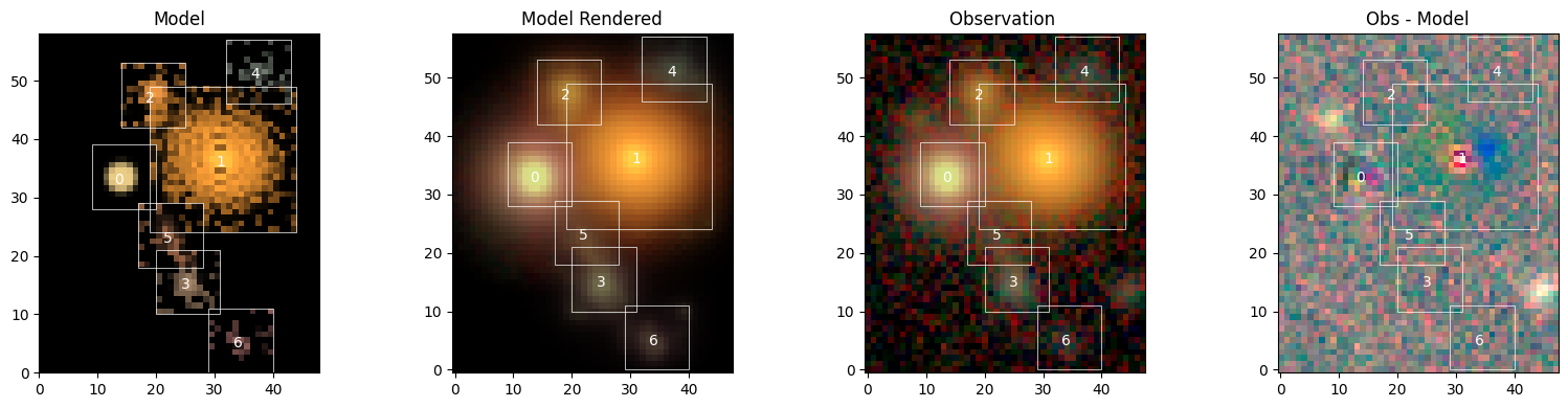
The fit is overall quite good, with low residuals, but it’s not perfect. Let’s investigate…
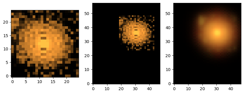
Access All Sources#
Individual sources can be accessed and evaluated as well, but we have to decide in which frame we want to see them. There are three options:
# Get models for source 1
source = scene_.sources[1]
# in its own source box (indicated by the white boxes in the figure above)
source_array = source()
# inserted in model frame
source_in_scene_array = scene_.evaluate_source(source)
# as it appears in observed frame
source_as_seen = obs.render(source_in_scene_array)

import matplotlib

# for imshow: don't interpolate the pixels, put origin to bottom
matplotlib.rc("image", interpolation="none", origin="lower")

fig, axes = plt.subplots(1, 3, figsize=(10, 4))
axes[0].imshow(sc2.plot.img_to_rgb(source_array, norm=norm))
axes[1].imshow(sc2.plot.img_to_rgb(source_in_scene_array, norm=norm))
axes[2].imshow(sc2.plot.img_to_rgb(source_as_seen, norm=norm))
plt.show()
We also provide a function to create all of these source images:
sc2.plot.sources(
    scene_,
    norm=norm,
    observation=obs,
    show_model=True,
    show_rendered=True,
    show_observed=True,
    show_spectrum=True,
    add_labels=False,
    add_boxes=True,
)
plt.show()
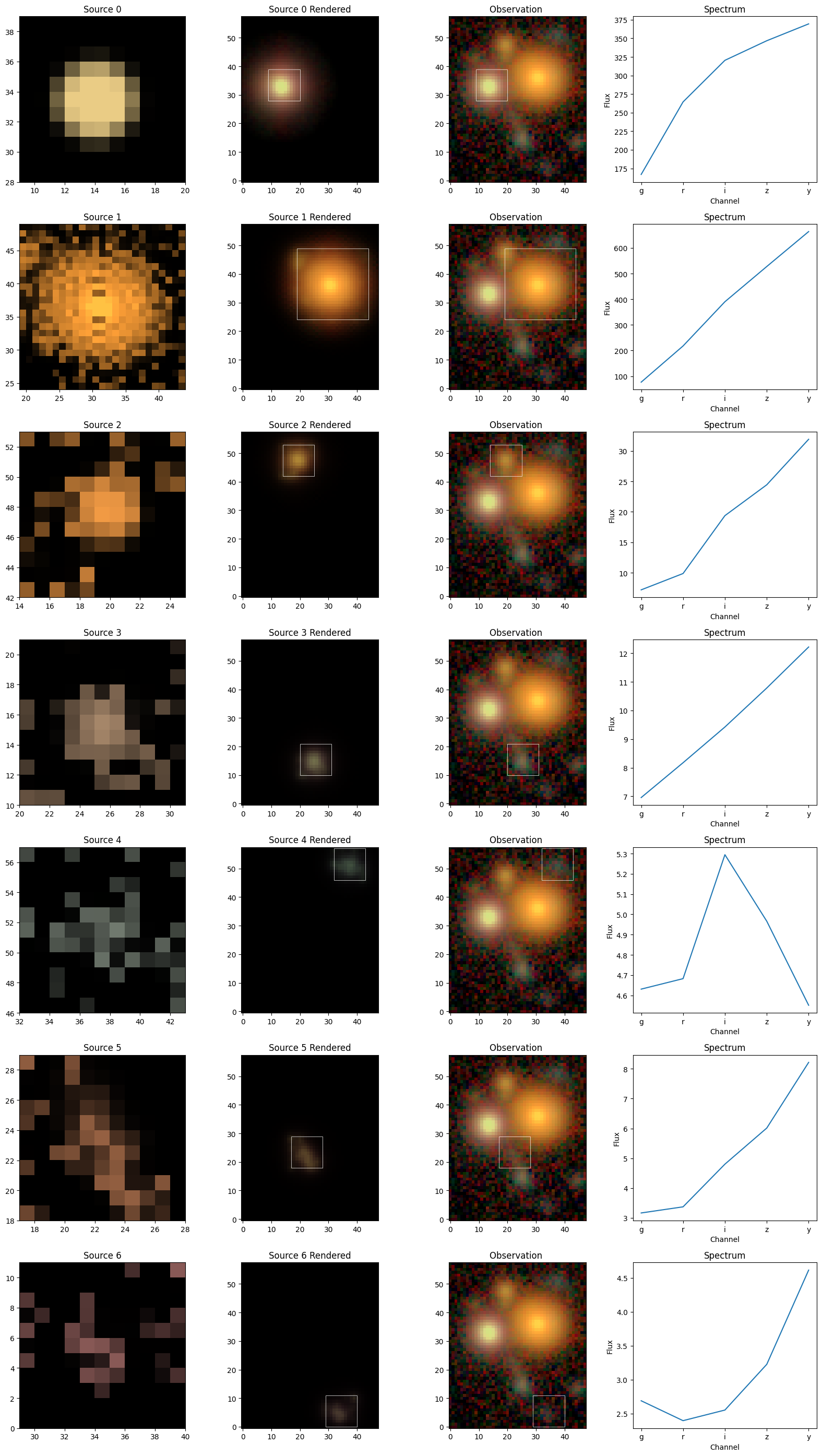
We can see that each source “lives” in a smaller box and is then placed into the larger scene. The model of object 0 assumes the simple Gaussian shape of the model PSF, which is the internal representation of a point source.
It’s noticeable that all other sources, however, show pixel patterns that don’t seem right. Some of them follow other sources (especially source 1) or noise (sources 4-6). What we see here is the limitation of non-parametric models: they can fit anything, but the likelihood may not have enough information to constrain all of these degrees of freedom. More/stronger constraints or priors can help, and we will describe their use in a separate tutorial.
Source Measurements#
As shown above, source models are generated in the model frame (dah…), from which any measurement can directly be made without having to deal with noise, PSF convolution, overlapping sources, etc.
For instance, the color information in these plots stems from the spectrum, i.e. the per-band amplitude, which are computed from the hyperspectral model by integrating over the morphology. The source spectra plots in the right panels above have done exactly that. The convention of these fluxes is given by the units and ordering of the original data cube.
print("----------------- {}".format(channels))
for k, src in enumerate(scene_.sources):
    print("Source {}, Fluxes: {}".format(k, sc2.measure.flux(src)))
----------------- ['g', 'r', 'i', 'z', 'y']
Source 0, Fluxes: [166.85814 264.4442  320.40704 346.77002 369.43085]
Source 1, Fluxes: [ 76.660706 217.68343  390.16125  527.5306   663.63586 ]
Source 2, Fluxes: [ 7.183556  9.865811 19.375763 24.448269 31.921381]
Source 3, Fluxes: [ 6.9573007  8.1738405  9.423243  10.786226  12.219091 ]
Source 4, Fluxes: [4.6312237 4.6828475 5.2944326 4.9660735 4.5516243]
Source 5, Fluxes: [3.1633193 3.368699  4.8006725 6.0127826 8.215358 ]
Source 6, Fluxes: [2.687453  2.3942358 2.5505846 3.2247329 4.613427 ]
Other measurements (e.g. centroid) or Moments are also implemented:
g = sc2.measure.Moments(scene_.sources[1])
print("Source 1 ellipticity:", g.ellipticity)
Source 1 ellipticity: [[ 0.09192424  0.09192435  0.09192406  0.09192424  0.0919243 ]
 [-0.1443111  -0.14431106 -0.14431112 -0.1443111  -0.1443111 ]]
All of these measurements are ordered by channel, so the ellipticity above is listed as [[e1_g, e1_r, e1_i, e1_z, e1_y],[e2_g, e2_r, e2_i, e2_z, e2_y]]. That they are all the same should not come as a surprise: For single-component models, there is no variation of the morphology across the channels.
Save and Re-Use Model#
To preserve the model for posterity, individual sources (or their sub-models) or entire scenes can be serialized into a HDF5 file:
import scarlet2.io as io

scene_id = 35
filename = "hsc_cosmos.h5"
io.model_to_h5(scene_, filename, id=scene_id, overwrite=True)
The stored model be loaded in the same way. Every source can be utilized as before.
scene__ = io.model_from_h5(filename, id=scene_id)
sc2.plot.scene(scene__, observation=obs, norm=norm, add_boxes=True)
plt.show()
We will now add two more sources to account for the largest residuals we have seen above. As we don’t know their location accurately, we allow the fitter to shift/recenter the sources.
# enter the context of the scene to create new elements
with scene__:
    # add two marginally detected sources at their approximate locations
    yx = [(14.0, 44.0), (42.0, 9.0)]
    for center in yx:
        center = jnp.array(center)
        # initialized like a point source
        spectrum = sc2.init.pixel_spectrum(obs, center)
        morph = sc2.init.compact_morphology()
        sc2.Source(center, spectrum, morph)

# need to remake the parameter structure including the new sources parameters
with sc2.Parameters(scene__) as params:
    # we could repeat the parameter definition from above
    # or: copy the parameters from scene
    params.update(scene.parameters)
    # define Parameter(s) for the new sources
    for i in range(len(scene.sources), len(scene__.sources)):
        sc2.Parameter(
            scene__.sources[i].spectrum,
            name=f"spectrum:{i}",
            constraint=constraints.positive,
            stepsize=spec_step,
        )
        sc2.Parameter(
            scene__.sources[i].morphology,
            name=f"morph:{i}",
            constraint=constraints.unit_interval,
            stepsize=morph_step,
        )

scene___ = scene__.fit(obs, max_iter=maxiter, e_rel=1e-4)
Running validation checks on the fit of the scene for observation .
Fit validation results:
[000]   INFO    The model fit is good. | Context={'chi2': Array(1.1692476, dtype=float32)})
[001]   WARN    The chi-square in the box for source 0 is acceptable, but not optimal. | Context={'chi2_in': Array(2.2541308, dtype=float32), 'source': 0})
[002]   INFO    The chi-square in the border for source 0 is good. | Context={'chi2_border': Array(0.93889195, dtype=float32), 'source': 0})
[003]   WARN    The chi-square in the box for source 1 is acceptable, but not optimal. | Context={'chi2_in': Array(1.623302, dtype=float32), 'source': 1})
[004]   INFO    The chi-square in the border for source 1 is good. | Context={'chi2_border': Array(1.065742, dtype=float32), 'source': 1})
[005]   INFO    The chi-square in the box for source 2 is good. | Context={'chi2_in': Array(0.9201341, dtype=float32), 'source': 2})
[006]   INFO    The chi-square in the border for source 2 is good. | Context={'chi2_border': Array(1.1433736, dtype=float32), 'source': 2})
[007]   INFO    The chi-square in the box for source 3 is good. | Context={'chi2_in': Array(1.0396882, dtype=float32), 'source': 3})
[008]   INFO    The chi-square in the border for source 3 is good. | Context={'chi2_border': Array(0.95360935, dtype=float32), 'source': 3})
[009]   INFO    The chi-square in the box for source 4 is good. | Context={'chi2_in': Array(0.82745117, dtype=float32), 'source': 4})
[010]   INFO    The chi-square in the border for source 4 is good. | Context={'chi2_border': Array(1.0198089, dtype=float32), 'source': 4})
[011]   INFO    The chi-square in the box for source 5 is good. | Context={'chi2_in': Array(0.9634988, dtype=float32), 'source': 5})
[012]   INFO    The chi-square in the border for source 5 is good. | Context={'chi2_border': Array(1.145741, dtype=float32), 'source': 5})
[013]   INFO    The chi-square in the box for source 6 is good. | Context={'chi2_in': Array(0.93531364, dtype=float32), 'source': 6})
[014]   INFO    The chi-square in the border for source 6 is good. | Context={'chi2_border': Array(1.0512719, dtype=float32), 'source': 6})
[015]   INFO    The chi-square in the box for source 7 is good. | Context={'chi2_in': Array(0.7987082, dtype=float32), 'source': 7})
[016]   INFO    The chi-square in the border for source 7 is good. | Context={'chi2_border': Array(0.9657884, dtype=float32), 'source': 7})
[017]   INFO    The chi-square in the box for source 8 is good. | Context={'chi2_in': Array(0.85000694, dtype=float32), 'source': 8})
[018]   INFO    The chi-square in the border for source 8 is good. | Context={'chi2_border': Array(1.3064857, dtype=float32), 'source': 8})
We can see that the fit is slightly better than before. Let’s have a look at the new model:
sc2.plot.scene(
    scene___,
    obs,
    norm=norm,
    show_model=True,
    show_rendered=True,
    show_observed=True,
    show_residual=True,
    add_boxes=True,
)
plt.show()
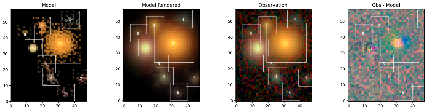
We can see the two new sources 7 and 8, and that most of the other features are very similar to before. As expected, the residuals have visibly improved where we added the source and are now dominated by a red-blue pattern in the center of source 1, which we should probably fit with 2 components.
Notice in plot on the right, source 0 has a slight color dipole close to the center. If you’ll recall when we created the Observation object a validation check produced an error that indicated misaligned PSF centroids. That PSF centroid misalignment is the likely cause of the dipole.