Fit Correlated Noise

This tutorial shows how to model sources from images that have been resampled or coadded and therefore now exhibit pixel correlations. We’ll demonstrate with an example from HST COSMOS coadds.

import astropy.io.fits as fits
import astropy.units as u
# Import Packages
import jax.numpy as jnp
from astropy.coordinates import SkyCoord
from astropy.table import Table
from astropy.wcs import WCS

import scarlet2 as sc2

sc2.set_validation(False)

Load Data

from huggingface_hub import hf_hub_download

filename = hf_hub_download(
    repo_id="astro-data-lab/scarlet-test-data",
    filename="multiresolution_tutorial/data.fits.gz",
    repo_type="dataset",
)

with fits.open(filename) as hdul:
    # Load HST observation
    data_hst = jnp.array(hdul["HST_OBS"].data, jnp.float32)
    wcs_hst = WCS(hdul["HST_OBS"].header)

    # Load HST PSF and weights
    psf_hst_data = jnp.array(hdul["HST_PSF"].data, jnp.float32)
    obs_hst_weights = jnp.array(hdul["HST_WEIGHTS"].data, jnp.float32)

    # Load catalog table and metadata
    coords_table = Table(hdul["CATALOG"].data)
    radecsys = hdul["CATALOG"].header["RADECSYS"]
    equinox = hdul["CATALOG"].header["EQUINOX"]

# Write sources coordinates in SkyCoord
ra_dec = SkyCoord(
    ra=coords_table["RA"] * u.deg,
    dec=coords_table["DEC"] * u.deg,
    frame=radecsys.lower(),
    equinox=f"J{equinox}",
)

Create Frame and Observations

We follow the usual pattern of creating an Observation and the model Frame.

# Scarlet Observations
obs_hst = sc2.Observation(
    data_hst, wcs=wcs_hst, psf=psf_hst_data, channels=["F814W"], weights=obs_hst_weights,
)
model_frame = sc2.Frame.from_observations(observations=obs_hst)
obs_hst.match(model_frame)
norm_hst = sc2.plot.AsinhAutomaticNorm(obs_hst)
sc2.plot.observation(obs_hst, sky_coords=ra_dec, label_kwargs={"color": "red"});

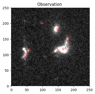
The noise fluctuations are larger than a single pixel, which means that neighboring pixel values are correlated. For comparison, this is how an uncorrelated noise field with the same variance would look like:

import jax
import matplotlib.pyplot as plt

key = jax.random.key(0)
noise_field = jax.random.normal(key, shape=obs_hst.data.shape) / jnp.sqrt(obs_hst.weights)
plt.imshow(sc2.plot.img_to_rgb(noise_field, norm=norm_hst))

<matplotlib.image.AxesImage at 0x70a7449e7340>

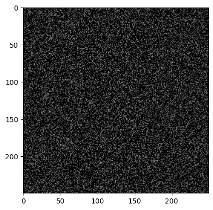
Were we to use the standard likelihood from Observation, we’d assume uncorrelated pixels and then overfit the data because we’d claim that features larger than a pixel could only arise from astrophysical sources when they can arise due to the resampling. To be clear, the correlations are everywhere, they are only easiest to see in the noisy regions.

We can create a modified observation, called CorrelatedObservation, which measures the pixel correlation in a patch of the image that contains as few sources as possible. It uses the correlation function to adjust the likelihood computation. Other than that, it behaves like any ordinary Observation.

obs_corr = sc2.CorrelatedObservation.from_observation(obs_hst)
obs_corr.match(model_frame)

Define sources and parameters

The parameters of the model follow our quickstart recommendations. The initialization routines could use either obs_hst or obs_corr because the data portion of these observations is identical; only the noise model is different.

with sc2.Scene(model_frame) as scene:
    for i, center in enumerate(ra_dec):
        try:
            spectrum, morph = sc2.init.from_gaussian_moments(obs_hst, center, min_snr=2)
        except ValueError:
            spectrum = sc2.init.pixel_spectrum(obs_hst, center)
            morph = sc2.init.compact_morphology()
        sc2.Source(center, spectrum, morph)

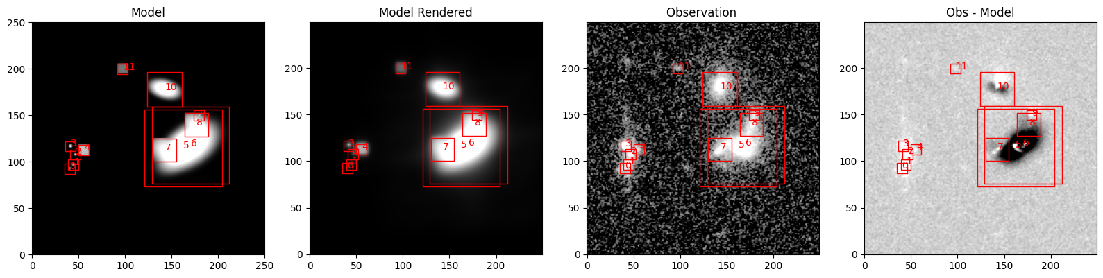
sc2.plot.scene(
    scene,
    observation=obs_hst,
    show_rendered=True,
    show_observed=True,
    show_residual=True,
    norm=norm_hst,
    add_boxes=True,
    label_kwargs={"color": "red"},
    box_kwargs={"edgecolor": "red", "facecolor": "none"},
);

from numpyro.distributions import constraints
from functools import partial

spec_step = partial(sc2.relative_step, factor=0.05)
morph_step = partial(sc2.relative_step, factor=1e-3)

with sc2.Parameters(scene):
    for i in range(len(scene.sources)):
        sc2.Parameter(
            scene.sources[i].spectrum,
            name=f"spectrum.{i}",
            constraint=constraints.positive,
            stepsize=spec_step
        )
        sc2.Parameter(
            scene.sources[i].morphology,
            name=f"morph.{i}",
            constraint=constraints.unit_interval,
            stepsize=morph_step,
        )

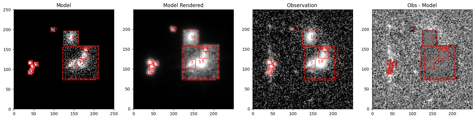
Fitting the model

We start with the uncorrelated noise model.

scene_ = scene.fit(obs_hst, max_iter=1000, e_rel=1e-4)

sc2.plot.scene(
    scene_,
    observation=obs_hst,
    show_rendered=True,
    show_observed=True,
    show_residual=True,
    add_labels=True,
    add_boxes=True,
    norm=norm_hst,
    box_kwargs={"edgecolor": "red", "facecolor": "none"},
    label_kwargs={"color": "red"},
);

A pretty decent fit, but there are some problems left. The model is missing flux around source 10 and the group of sources 0-4 in the left because the boxes are too narrow. We can also see that the model picks up a lot of noise fluctuations. While one cannot rule out that some of them correspond to actual source emission, the residuals on the right show that the model is overfitting: the structure in the region of source 5 and 6 is much flatter (and importantly: shows smaller scale residuals) than in other regions.

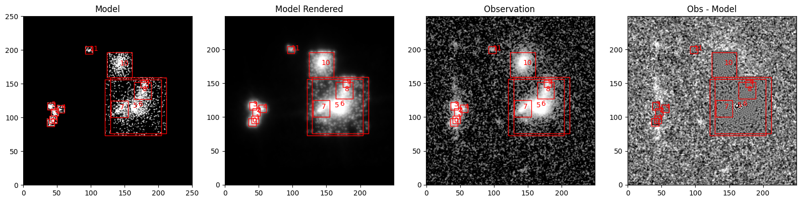
Now we repeat the same process with the CorrelatedObservation we created earlier:

scene_corr = scene.fit(obs_corr, max_iter=1000, e_rel=1e-4)

sc2.plot.scene(
    scene_corr,
    observation=obs_hst,
    show_rendered=True,
    show_observed=True,
    show_residual=True,
    add_labels=True,
    add_boxes=True,
    norm=norm_hst,
    box_kwargs={"edgecolor": "red", "facecolor": "none"},
    label_kwargs={"color": "red"},
);

The residuals are more “grainy” now and look more consistent with the noise in other areas. In the region of sources 5 and 6, the model is still overfitting, but that’s because we fit two sources to a single-band image. Such a fit is underconstrained and therefore prone to overfitting. Using additional observations in other filters can help (provided that sources 5 and 6 have different SEDs). See the multi-observation tutorial for details.