Fit Multiple Observations

This tutorial shows how to model sources from images observed in different ways, which could mean images taken with the same instrument but different pointings and PSFs, or with different instruments. For this guide we will use a multi-band observation from the Hyper-Suprime Cam (HSC) and a single high-resolution image from the Hubble Space Telescope (HST).

# Import Packages
import astropy.io.fits as fits
import astropy.units as u
import jax.numpy as jnp
from astropy.coordinates import SkyCoord
from astropy.table import Table
from astropy.wcs import WCS

import scarlet2 as sc2
sc2.set_validation(False)

Load Data

We first load the HSC and HST images, PSFs and weight/variance maps and store them in their own Observation instances. We also load a catalog of sources detected jointly from the observations (see here for details on how this catalog was created).

from huggingface_hub import hf_hub_download

filename = hf_hub_download(
    repo_id="astro-data-lab/scarlet-test-data",
    filename="multiresolution_tutorial/data.fits.gz",
    repo_type="dataset",
)
with fits.open(filename) as hdul:
    # Load two Observations
    obs_hst = sc2.Observation(
        # Data amplitude is ~10x larger in HST as in HSC
        # For better optimization: adjustment data and variance
        # details at https://github.com/pmelchior/scarlet2/issues/240
        hdul["HST_OBS"].data / 10,
        weights=hdul["HST_WEIGHTS"].data * 100,
        psf=hdul["HST_PSF"].data,
        wcs=WCS(hdul["HST_OBS"].header),
        channels=["F814W"],
        name="HST",
    )
    obs_hsc = sc2.Observation(
        hdul["HSC_OBS"].data,
        weights=hdul["HSC_WEIGHTS"].data,
        psf=hdul["HSC_PSF"].data,
        channels=["g", "r", "i", "z", "y"],
        wcs=WCS(hdul["HSC_OBS"].header),
        name="HSC",
    )

    # Load source catalog
    coords_table = Table(hdul["CATALOG"].data)
    radecsys = hdul["CATALOG"].header["RADECSYS"]
    equinox = hdul["CATALOG"].header["EQUINOX"]
    ra_dec = SkyCoord(
        ra=coords_table["RA"] * u.deg,
        dec=coords_table["DEC"] * u.deg,
        frame=radecsys.lower(),
        equinox=f"J{equinox}",
    )

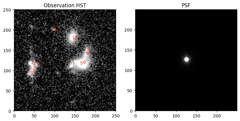
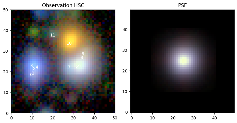
Now we display the observation contents:

norm_hst = sc2.plot.AsinhAutomaticNorm(obs_hst)
norm_hsc = sc2.plot.AsinhAutomaticNorm(obs_hsc)

sc2.plot.observation(
    obs_hst,
    norm=norm_hst,
    add_peaks=ra_dec,
    show_psf=True,
    label_kwargs={"color": "red"}
);
sc2.plot.observation(
    obs_hsc,
    norm=norm_hsc,
    add_peaks=ra_dec,
    show_psf=True
);

Define Model Frame and Resample

As we have two different instruments with different pixel resolutions, we need define a model frame that allows us to jointly model these data:

model_frame = sc2.Frame.from_observations(
    observations=[obs_hst, obs_hsc],
    coverage="union",  # or "intersection"
)

This method defines a common area for both observations, in this case a box covering the union of both. Doing so allows to fit sources as long as at least one of the observation has valid pixels. To enforce homogeneous coverage, use coverage="intersection". In addition, the model frame adopts the HST resolution because the HST image has the highest resolution. The channels of both observations are simply concatenated, which means the bands are treated independently across observations, even though the wavelengths may overlap.

We could initialize the needed parameter and simply call:

sc2.fit(scene, [obs_hst, obs_hsc], max_iter=1000, progress_bar=True)

And this would work, but it would take a long time. The rendering operator for the HSC observation has to change resolution. This operation is much slower than, say, a simple convolution at the same resolution. We therefore resample the HSC observation to the pixel grid of the model frame (which has inherited its pixel grid from the HST observation):

obs_hsc_corr = sc2.CorrelatedObservation.from_observation(obs_hsc, resample_to_frame=model_frame)
obs_hsc_corr.match(model_frame)
norm_hsc_corr = sc2.plot.AsinhAutomaticNorm(obs_hsc_corr)
sc2.plot.observation(obs_hsc_corr, norm=norm_hsc_corr, add_peaks=ra_dec, show_psf=True);

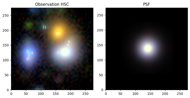
The new observation does not require resampling during the fit. And because the resampling correlates the pixel values, we automatically treat it as a CorrelatedObservation.

For good measure, we should also account for the pixel correlations in the HST data, which arose because the HST single exposures were also resampled when the HST coadd was created (see the tutorial on correlated data for more details). Since the HST and the model frame share the same pixel grid, we don’t need to resample to the model frame here:

obs_hst_corr = sc2.CorrelatedObservation.from_observation(obs_hst)

Initialize Sources from Multiple Observations

The initialization of the sources follows our general recommendation (from e.g. the quickstart guide):

with sc2.Scene(model_frame) as scene:
    infos = sc2.init.hierarchical_sources(
        obs_hst,
        K=3,
        scales=[1,2,3],
        min_area=16,
        strict=True,
        catalog=ra_dec,
        split_peaks=False,
        image_type="space"
    )
    for sinfo in infos:
        sc2.Source(sinfo.center, sinfo.spectrum, sinfo.morphology)

We chose the HST image for the initialization because it has the higher resolution and should therefore be able to better identify the position and shape of the sources. We also set split_peaks=False because the sources (especially the groups 0-4 and 7-9) definitely overlap, so we want to allow the footprints to overlap as well. And because the space-based PSF wodth is on the order of 1 pixel, the multi-scale support calculation needs to be adjusted with image_type="space".

So far we know nothing about the source spectra in the HSC bands. But we can use the HST-defined morphology to perform forced photometry in the HSC bands. We put the measured fluxes in the appropriate channels of the spectra:

hsc_spectra = sc2.measure.forced_photometry(scene, obs_hsc_corr)
channel_map = model_frame.map_channels(obs_hsc_corr.frame)
for i in range(len(scene.sources)):
    spectrum = scene.sources[i].spectrum
    for model_channel, obs_channel in channel_map.items():
        spectrum = spectrum.at[model_channel].set(hsc_spectra[i, obs_channel])
    scene.sources[i] = scene.sources[i].replace("spectrum", spectrum)

sc2.plot.scene(
    scene,
    observation=obs_hst,
    show_rendered=True,
    show_observed=True,
    show_residual=True,
    add_labels=True,
    add_boxes=True,
    norm=norm_hst,
    box_kwargs={"edgecolor": "red", "facecolor": "none"},
    label_kwargs={"color": "red"},
)
sc2.plot.scene(
    scene,
    observation=obs_hsc_corr,
    show_rendered=True,
    show_observed=True,
    show_residual=True,
    add_labels=True,
    add_boxes=True,
    norm=norm_hsc_corr,
    label_kwargs={"color": "red"},
);

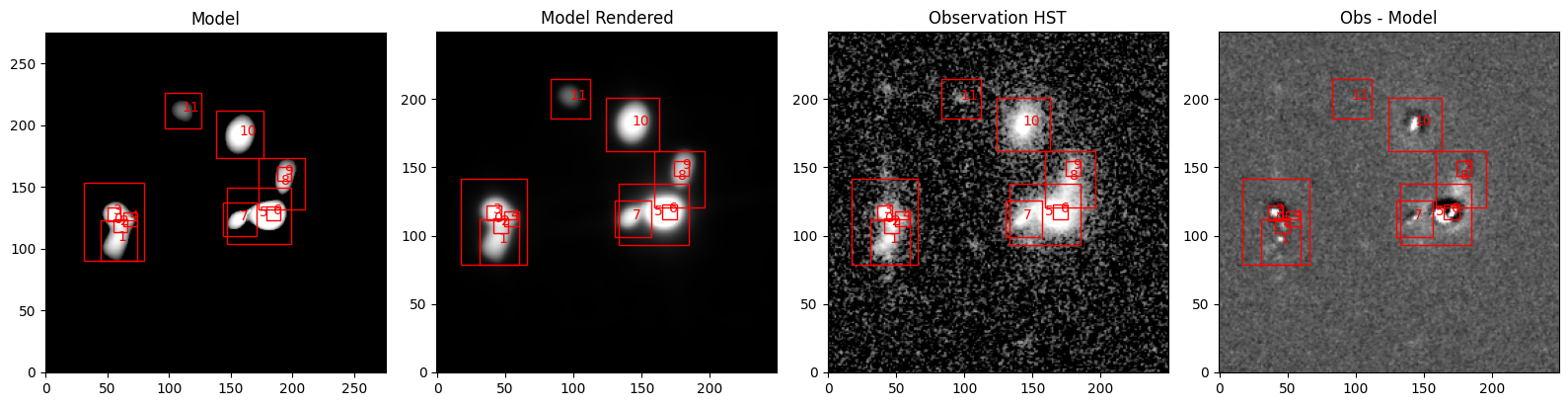
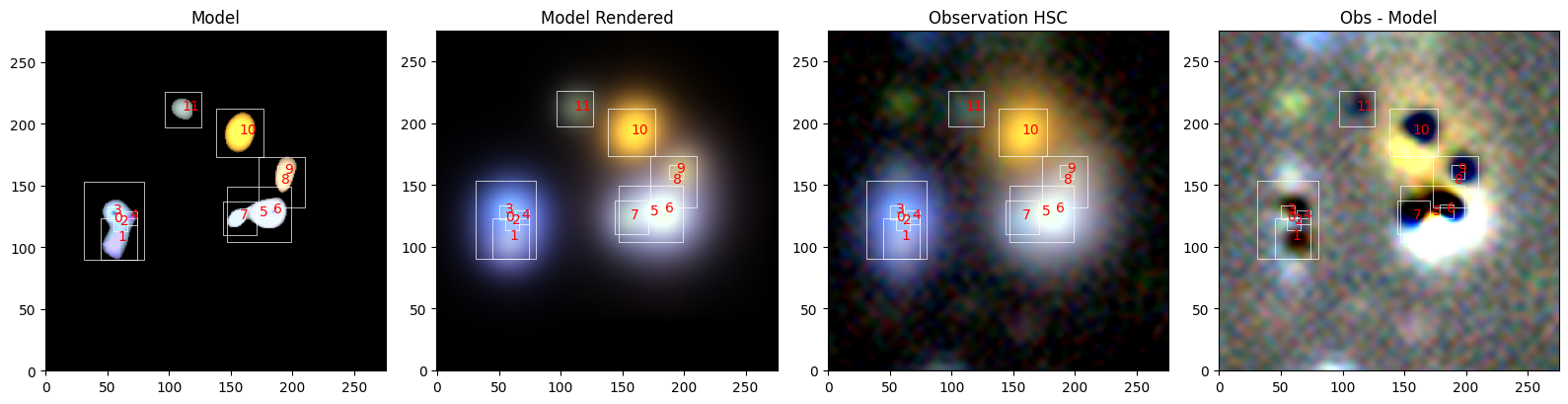
That’s a pretty reasonable initialization, so let’s proceed with the usual parameter definition:

from functools import partial
from numpyro.distributions import constraints

# best step size for parameters with a relative "uncertainty":
# big/bright sources adjust more quickly
spec_step = partial(sc2.relative_step, factor=0.05)
morph_step = 0.1

with sc2.Parameters(scene):
    for i in range(len(scene.sources)):
        # because we want the spectrum parameter to be constrained,
        # we need to ensure that their initialization satisfies the constraint
        tiny = 1e-6
        spectrum = scene.sources[i].spectrum
        if (spectrum <= 0).any():
            scene.sources[i] = scene.sources[i].replace("spectrum", jnp.maximum(spectrum, tiny))
        sc2.Parameter(
            scene.sources[i].spectrum,
            name=f"spectrum:{i}",
            constraint=constraints.positive,
            stepsize=spec_step,
        )
        # same for [0,1] constrained morphology
        morph = spectrum = scene.sources[i].morphology
        if ((morph <= 0) | (morph >= 1)).any():
            scene.sources[i] = scene.sources[i].replace("morphology", jnp.clip(morph, tiny, 1-tiny))
        sc2.Parameter(
            scene.sources[i].morphology,
            name=f"morph:{i}",
            constraint=constraints.unit_interval,
            stepsize=morph_step,
        )

We can now pass both observations to the fitting method:

scene_ = scene.fit([obs_hst_corr, obs_hsc_corr], max_iter=1000, progress_bar=True)

Let’s check the results:

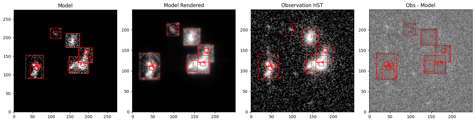
sc2.plot.scene(
    scene_,
    observation=obs_hst_corr,
    show_rendered=True,
    show_observed=True,
    show_residual=True,
    add_labels=True,
    add_boxes=True,
    norm=norm_hst,
    box_kwargs={"edgecolor": "red", "facecolor": "none"},
    label_kwargs={"color": "red"},
)
sc2.plot.scene(
    scene_,
    observation=obs_hsc_corr,
    show_rendered=True,
    show_observed=True,
    show_residual=True,
    add_labels=True,
    add_boxes=True,
    norm=norm_hsc_corr,
);

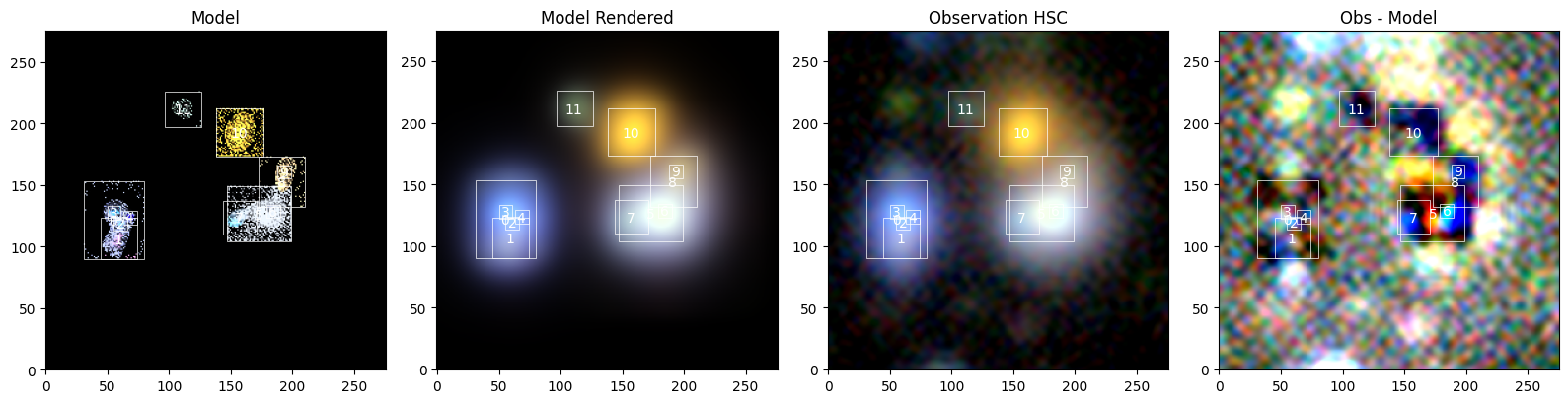
The fit is quite good, but issues remain:

• The model is still quite noisy in the outskirts. We are currently developing morphology priors for space-based imaging which should improve the reconstruction fidelity.

• The boxes are too small, so some flux, e.g. around source 10, is not modeled. That’s a consequence of the shallower surface brightness limit of the HST image: it misses the outskirts of the sources, which are visible in the HSC residuals.

• There are minor dipoles in the residuals (best seen for source 10), which skew in the opposite directions between the two observations (the top-right is positive in HST, while the top-right is negative in HSC). That could imply that the astrometry between the HSC and HST is slightly inconsistent.

Let’s see how we can fix that:

Fit Astrometric Offsets

We can treat this offset by understanding that each observation has a Renderer, which maps the modeled scene onto the observation. The figures above show this operation in the column called “Model Rendered”. The renderers here perform a convolution and have an attribute .shift, which, well, shifts the convolved image. We can use this attribute as a Parameter, which means that we treat the observation as a model that can be optimized, just like scene.

Tip

Because the astrometric offset is relative, it’s sufficient to only shift one observation (or more precisely: all but one). The observation whose shift we do not adjust thus defines the astrometric reference. Without this fixed anchor, all observations can be shifted by an arbitary amount, which would make the fitter or sampler unhappy: it’s a perfect degeneracy.

So let’s define the shift parameter for the HSC observation only, and fit the same scene again. As we will update scene and observations, we need the more flexible fitting function scarlet2.fit() rather than scene.fit.

# making sure that the renderer exists
obs_hsc_corr.check_set_renderer(model_frame)

# define shift parameter: unconstrained, with milli-arcsec stepsize
import astropy.units as u

with sc2.Parameters(obs_hsc_corr):
    sc2.Parameter(obs_hsc_corr.renderer[1].shift, name="shift", stepsize=1e-3 * u.arcsec)

# the more flexible fitter optimizes scene and observations and returns both
scene_, (_, obs_hsc_corr_) = sc2.fit(scene_, [obs_hst_corr, obs_hsc_corr], e_rel=1e-4, max_iter=1000)

# get the astrometry shift
shift = obs_hsc_corr_.get("shift")
print(f"Shift in model pixels: {shift}")

Shift in model pixels: [-0.77367556 -0.38265565]

The fit is slightly better than before, but let’s see if the models look better:

sc2.plot.scene(
    scene_,
    observation=obs_hst_corr,
    show_rendered=True,
    show_observed=True,
    show_residual=True,
    add_labels=True,
    add_boxes=True,
    norm=norm_hst,
    box_kwargs={"edgecolor": "red", "facecolor": "none"},
    label_kwargs={"color": "red"},
)
sc2.plot.scene(
    scene_,
    observation=obs_hsc_corr_,
    show_rendered=True,
    show_observed=True,
    show_residual=True,
    add_labels=True,
    add_boxes=True,
    norm=norm_hsc_corr,
);

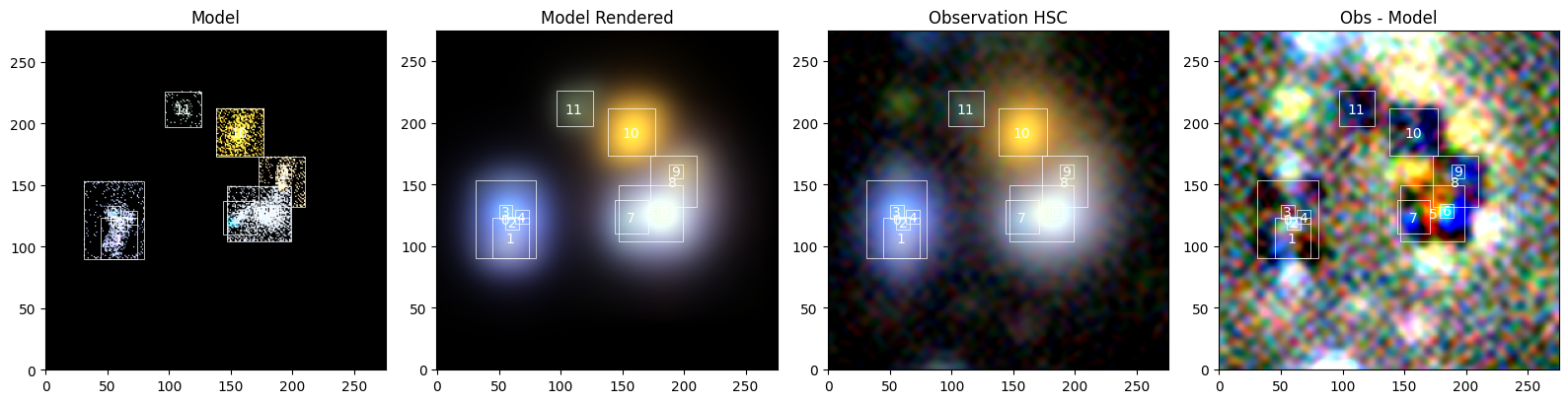
The dipoles have indeed vanished. The residuals, especially for HSC, are now dominated by the outskirts of galaxies (especially #10) and previously undetected sources, missing from the reference catalog ra_dec. If we want to improve the fits, we need joint detection/initialization.

Evaluate in Native Resolution

This leaves us with only last question: We have fit the resampled HSC observation, but does the model actually describe the original HSC data?

We can simply plot scene_ against the original obs_hsc, but we wouldn’t get the correction for the astrometric offset, which is a parameter of obs_hsc_corr. In addition, we need to use the WCSs of the observations to compute the shift in native HSC pixels rather than the resampled observation we fit:

# get the Jacobian transform between the resampled and native HSC frame
jacobian, _ = sc2.frame.get_relative_jacobian_shift(obs_hsc_corr_.frame, obs_hsc.frame)
shift_native = jacobian @ shift
print(f"Shift in native HSC pixels: {shift_native}")

# create the renderer for native HSC if not already there
obs_hsc.check_set_renderer(model_frame)
# force the renderer to use optimized value for shift
object.__setattr__(obs_hsc.renderer[-1], "shift", shift_native)

Shift in native HSC pixels: [-0.13815634 -0.06833136]

This is a pretty small shift, which may have been caused by differences in the stellar catalog used to define the astrometry in each observation or the centering algorithm for the PSF models. But let’s check out the model compared to the original HSC observation:

sc2.plot.scene(
    scene_,
    observation=obs_hsc,
    show_rendered=True,
    show_observed=True,
    show_residual=True,
    add_labels=True,
    add_boxes=True,
    norm=norm_hsc,
);

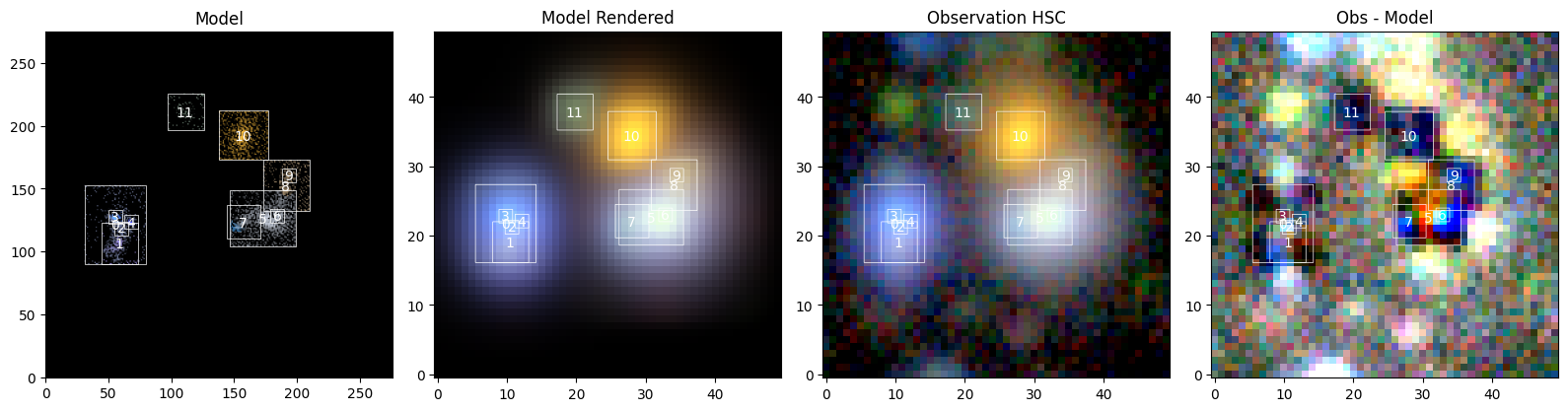
So, does a model trained on resampled data provide a good fit for the native data? Yeah, it does!