Fit a Low Surface Brightness Galaxy

This tutorial goes through a case where the many modeling codes struggle: a well-resolved galaxy with lots of internal structure and low-surface brightness (LSB) emission.

# Import Packages and setup
import jax.numpy as jnp
import matplotlib.pyplot as plt
import scarlet2 as sc2
import pickle

sc2.set_validation(False)

import matplotlib
# use a suitable colormap and don't interpolate the pixels
matplotlib.rc('image', interpolation='none', origin="lower", cmap="inferno")

Load and Display Data

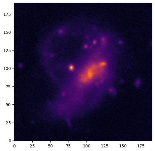
We load the data set (an image cube from HSC with 5 bands):

# Load the sample images
from huggingface_hub import hf_hub_download

filename = hf_hub_download(
    repo_id="astro-data-lab/scarlet-test-data",
    filename="lsbg.pkl",
    repo_type="dataset"
)
data= pickle.load(open(filename, "rb"))
images = data["images"]
channels = data["channels"]
psf = data["psfs"]

plt.figure(figsize = (6,6))
plt.imshow(images.sum(axis=0))
plt.show()

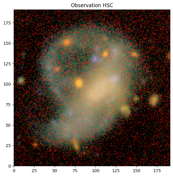
The data file does not contain any estimate of the noise level. So, we need to find a patch of “empty” sky to measure the noise. Gladly, the corners of the image show no apparent sources:

sky_patch = images[:, 150:, 150:]
variance = sky_patch.var(axis=(-2, -1))
variance = jnp.ones(images.shape) * variance[:,None,None]
obs = sc2.Observation(images, 1/variance, channels=channels, psf=psf, name="HSC")

norm = sc2.plot.AsinhAutomaticNorm(obs)
sc2.plot.panel_size = 6
sc2.plot.observation(obs, norm=norm);

Detect Sources

LSB features pose a particular challenge for source detection: the faint outer envelopes of galaxies only become significant at large wavelet scales, where compact objects are invisible. We therefore start by tuning the detection parameters for multiscale_footprints() to capture extended emission rather than splitting it up:

• strict=False: We want to perform detection not just in the scale-specific starlet images, but also in the large-scale remainder, where the LSB emission should be most apparent. If we set strict=True, most of the LSB contribution would be declared as background for detection purposes.

• split_peaks=False: Footprints with multiple peaks are kept intact. Splitting them would fragment the LSBG into many small sub-components, obscuring its true extent.

• K=2: A lower significance threshold than the default of 3 catches faint pixels that would otherwise be missed.

Passing return_intermediates=True gives us direct access to the wavelet coefficient images (detect) and the per-scale footprint dictionary (footprints) so we can inspect what was found at each scale:

scales = [1,2]
K=2
min_area=16
strict = False
split_peaks = False
detect, sigma, scales, footprints = sc2.detect.multiscale_footprints(
    obs,
    scales=scales,
    strict=strict,
    K=K,
    split_peaks=split_peaks,
    min_area=min_area,
    return_intermediates=True,
)

sc2.plot.footprints(detect, footprints);

print("Scale | FPs  | Peaks")
total, total_peaks = 0,0
for scale in scales:
    fps = len(footprints[scale])
    peaks = sum([len(fp.peaks) for fp in footprints[scale]])
    print(f"    {scale} | {fps:<4} | {peaks}")
    total += fps
    total_peaks += peaks
print("    ---------------")
print(f"      | {total:<4} | {total_peaks}")

Scale | FPs  | Peaks
    1 | 45   | 77
    2 | 4    | 26
    ---------------
      | 49   | 103

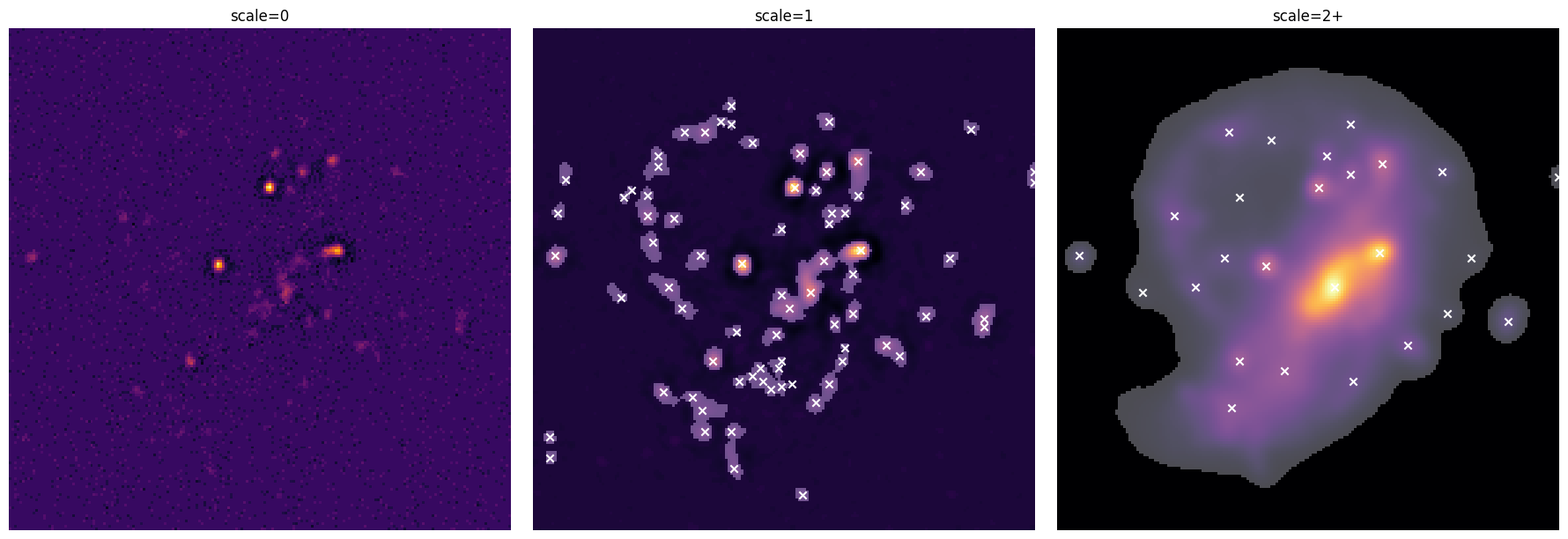
The plot shows the detection starlet coefficients at each scale, with detected footprint regions overlaid in grey and peaks marked as white crosses. The table summarizes how many independent footprints and peaks were found per scale. It is clear that scale 1 does most of the heavy lifting here, but scale 2 (and above because strict=False) nicely detects the large LSBG.

These per-scale footprints are still independent of one another, and some of the found peaks are duplicated across scales. hierarchical_footprints() links them into a unified source list: the largest-scale detection becomes the primary footprint for each source, and its peak position and extent are refined using the finer-scale detections:

footprints = sc2.detect.hierarchical_footprints(
    obs,
    scales=scales,
    strict=strict,
    K=K,
    min_area=min_area,
    split_peaks=split_peaks
)
sc2.plot.observation(obs, norm=norm, add_footprints=footprints, add_peaks=footprints, label_kwargs={"color": "red"});

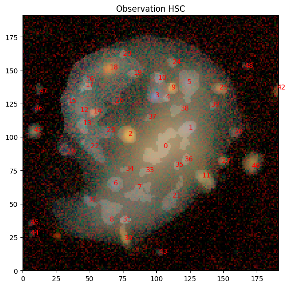
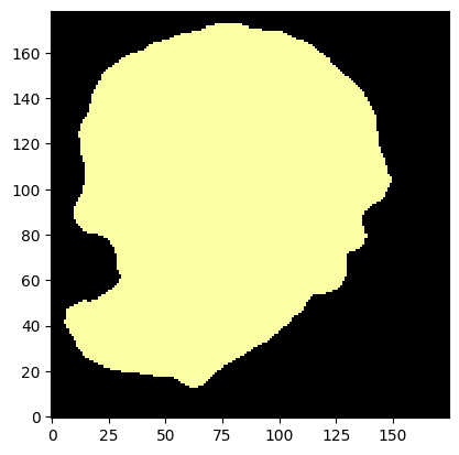
The red markers show the peak position of each detected source overlaid on the full observation. Source 0 should cover the full extent of the LSBG, including its low-surface-brightness outskirts. We can confirm this by inspecting its footprint mask directly:

plt.imshow(footprints[0].footprint);

Initialize Sources

With the detections in hand, we can build the Scene. The model frame is adapted from the observation, so that we match the different PSFs across bands.

hierarchical_sources() re-runs the same detection internally (using our preferred parameter values) and constructs an initial Source for each detected object:

model_frame = sc2.Frame.from_observations(obs)

with sc2.Scene(model_frame) as scene:
    infos = sc2.init.hierarchical_sources(
        obs,
        scales=scales,
        strict=strict,
        K=K,
        min_area=min_area,
        split_peaks=split_peaks
    )
    for sinfo in infos:
        sc2.Source(sinfo.center, sinfo.spectrum, sinfo.morphology)

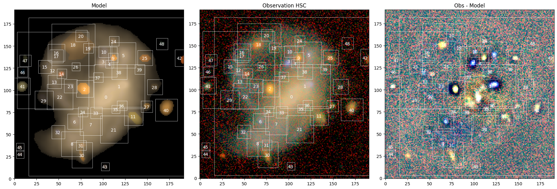
sc2.plot.scene(
    scene,
    observation=obs,
    norm=norm,
    show_observed=True,
    show_residual=True,
    add_boxes=True
);

Fit the Model

The initial models are a reasonable starting point, but the spectra and morphologies need to be refined through optimization. So, we register Parameter objects for every quantity we want the fitter to update.

from functools import partial
from numpyro.distributions import constraints

# reduce the spectrum step size from 0.05
# to stabilize massively overlapping sources
spec_step = partial(sc2.relative_step, factor=0.02)
morph_step = 0.1

with sc2.Parameters(scene):
    for i in range(len(scene.sources)):
        # because we want the spectrum parameter to be constrained,
        # we need to ensure that their initialization satisfies the constraint
        tiny = 1e-6
        spectrum = scene.sources[i].spectrum
        if (spectrum <= 0).any():
            scene.sources[i] = scene.sources[i].replace("spectrum", jnp.maximum(spectrum, tiny))
        sc2.Parameter(
            scene.sources[i].spectrum,
            name=f"spectrum:{i}",
            constraint=constraints.positive,
            stepsize=spec_step,
        )
        # same for [0,1] constrained morphology
        morph = spectrum = scene.sources[i].morphology
        if ((morph <= 0) | (morph >= 1)).any():
            scene.sources[i] = scene.sources[i].replace("morphology", jnp.clip(morph, tiny, 1-tiny))
        sc2.Parameter(
            scene.sources[i].morphology,
            name=f"morph:{i}",
            constraint=constraints.unit_interval,
            stepsize=morph_step,
        )

Because there is so extensive overlap between the sources, we add an additional penalty term as regularizer: PairSimilarity. It reduces the spatial similarity of two components with similar color (see details in the documentation). In other words, it will help separate sources in cases where the data likelihood alone cannot distinguish between them. The only downside is that this penalty is computed over all source pairs, of which we have many here, so there is a non-trivial runtime cost, but it’ll be worth it.

We use a small contribution of 1% of the reconstruction loss to aid with the separation without overwhelming the fit:

maxiter = 200
sim = sc2.PairSimilarity(weight=1e-2)
scene_ = scene.fit(obs, max_iter=maxiter, e_rel=1e-3, pair_similarity=sim)

scene_array = scene_()
print("Optimized chi^2:", obs.goodness_of_fit(scene_array))

Optimized chi^2: 1.0040114

sc2.plot.scene(
    scene_,
    obs,
    norm=norm,
    show_model=True,
    show_rendered=True,
    show_observed=True,
    show_residual=True,
    add_boxes=True,
);

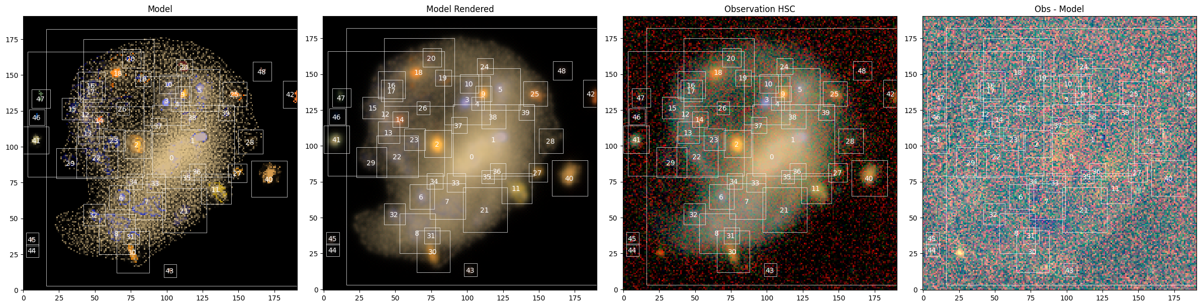
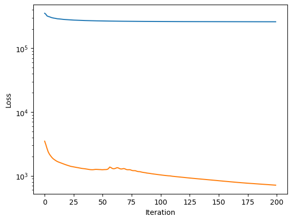
The residuals are small across most of the field, with mild deviations near the center of the LSBG, where the internal structure is most complex, and in the regions of overlap between sources. We can check the fit and the penalty improvements over the course of the fit:

plt.semilogy(scene_.fit_info['loss'])
plt.semilogy(scene_.fit_info['pair_similarity'])
plt.ylabel('Loss')
plt.xlabel('Iteration')
plt.show()

Inspecting the LSBG component

# Get models for source 0
source = scene_.sources[0]
# inserted in model frame
source_in_scene_array = scene_.evaluate_source(source)
# as it appears in observed frame
source_as_seen = obs.render(source_in_scene_array)
fig, ax = plt.subplots(1,2, figsize=(10,5))
ax[0].imshow(sc2.plot.img_to_rgb(source_as_seen, norm=norm))
ax[0].text(0.05, 0.95, 'LSBG', color='white', ha='left', va='top', transform=ax[0].transAxes)
ax[1].imshow(sc2.plot.img_to_rgb(obs.data - source_as_seen, norm=norm))
ax[1].text(0.05, 0.95, 'Residual', color='white', ha='left', va='top', transform=ax[1].transAxes)
plt.show()

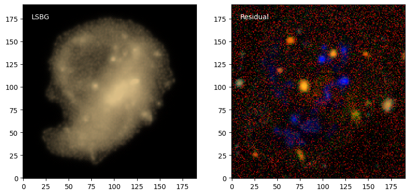
The LSBG model captures the extended low-surface-brightness emission and the core structure of the galaxy simultaneously. It’s still picking up some flux from other components, but the similarity regularizer we used has restricted it to relatively faint components with other colors.

It’s also quite grainy, a result of the low SNR of most of the LSB emission (that’s what the “L” stands for…). A morphology model, like StarletMorphology, with suitable priors on the coefficients, should be well-suited here (see issue #250 for ideas) and make the regularizer even more effective.

Because the model is evaluated in a clean, noise-free, deblended frame, any photometric or morphological measurement, such total flux, half-light radius, ellipticity, can now be made directly from source_model without PSF or neighbor contamination. See scarlet2.measure for the available measurement functions.