Detect Sources

This guide shows how to detect sources in an observation using wavelet techniques. The same approach can also be used to initialize sources for scene modeling. For this demonstration, we’ll closely follow the Real-World Example.

# Import Packages and setup
import jax.numpy as jnp
import matplotlib.pyplot as plt
import scarlet2 as sc2

# use a suitable colormap and don't interpolate the pixels
import matplotlib

from scarlet2.plot import panel_size

matplotlib.rc('image', interpolation='none', origin="lower", cmap="inferno")

Data Loading

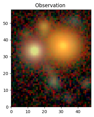
We load the example data set (a HSC 5-band image). It contains a detection catalog, but we will initially pretend it does not.

from huggingface_hub import hf_hub_download

filename = hf_hub_download(
    repo_id="astro-data-lab/scarlet-test-data",
    filename="hsc_cosmos_35.npz",
    repo_type="dataset"
)
file = jnp.load(filename)
data = file["images"]
channels = [str(f) for f in file["filters"]]
weights = 1 / file["variance"]
psf = file["psfs"]
catalog = jnp.array([(src["y"], src["x"]) for src in file["catalog"]])

Warning: You are sending unauthenticated requests to the HF Hub. Please set a HF_TOKEN to enable higher rate limits and faster downloads.

While some of the detection methods below work just fine on regular image arrays, working with Observation make many operations more convenient.

obs = sc2.Observation(data, weights=weights, psf=psf, channels=channels)

# display the observation
norm = sc2.plot.AsinhAutomaticNorm(obs)
sc2.plot.observation(obs, norm=norm);

Observation validation results:
[000]   INFO    Number of channels in the observation matches the data.
[001]   INFO    Data and weights have the same shape.
[002]   INFO    Observation.weights in the observation are finite and non-negative.
[003]   INFO    Data in the observation are finite where weights are greater than zero.
[004]   INFO    PSF is 3-dimensional.
[005]   INFO    Number of PSF channels matches the number of data channels.
[006]   WARN    PSF centroid is not the same in all channels. | Context={'psf_centroid': Array([[ 0.04197121, -0.01779556,  0.0002327 ,  0.04332542,  0.06899071],
       [ 0.09050751,  0.01180649, -0.03284836,  0.08525848, -0.00099373]],      dtype=float32)})

Starlets

We employ the starlet transformation, popularized by Starck, Murtagh & Bertero (2015), implemented in scarlet2.wavelets.starlet_transform(), to decompose the observation into different scales. In detail, the method scarlet2.detect.multiscale_footprints() combines all bands of the observation with inverse-variance weights into a 2D detection image, which then gets transformed into the starlet basis. At every scale, the resulting starlet coefficients form an image of the same shape as the original, but with increasingly larger spatial scales. The last scale contains everything that is not contained on smaller scales, which means that the transformation is exact (in fact, it’s overcomplete because there are multiple ways to represent the same input image). The method returns the coefficients with significant support across multiple scales. In this filtered image, called detect below, areas above some threshold should correspond to the sources we seek to find. The method then runs a flood-filling algorithm to find connected regions of a certain size: source footprints.

We visualize the results with scarlet2.plot.footprints():

detect, sigma, scales, footprints = sc2.detect.multiscale_footprints(
    obs,
    # starlets scales to compute
    scales=[1,2,3],
    # for strict scale separation: run detection only on scales above,
    # but add another scale for the residuals without detecting on it
    strict=True,
    # multiscale support threshold: K-sigma fluctuation across bands and scales
    K=2,
    # break apart peaks in the same footprint
    split_peaks=True,
    # for ground-based images PSF likely larger than scale 0, 1
    image_type="ground",
    # find compact regions of a minimum area above 0 in detection image:
    # footprints of detected source, shown as semi-transparent contours
    min_area=9,
    # return detect, sigma & scales, not just footprints
    return_intermediates=True,
)

sc2.plot.footprints(detect, footprints);

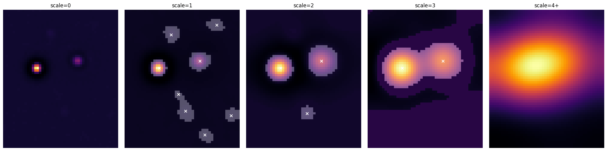
We can see that smaller scales allow smaller sources to be found, even in the presence of neighbors, whereas larger scales capture extended source emission (especially for the bright sources in this image).

Tip

Reducing K lets the algorithm find fainter sources, but makes it more vulnerable to noise fluctuations. Increasing min_area removes small fluctuations, but can reject small legitimate sources, too. When in doubt, run the code above on your data and tweak scales, strict, K, and min_area, until you are satisfied.

It’s clear that at any of these scales we find connected regions, aka “footprints”, above some threshold, and then find peaks within footprints. But a good detection method should be able to combine information across scales to deal with compact and extended sources.

Hierarchical Detection

For that, we have created a hierarchical detection method, scarlet2.detect.hierarchical_footprints(), which uses the same underlying starlet footprint approach, but then starts with the footprints found on the largest scale and adds those of all smaller scales. If a footprint on a smaller scale overlaps with a footprint on a larger scale but is offset from the larger-scale peak, it is added as child of the larger footprint. Footprints within footprints… Which makes a lot of sense for complex or blended sources.

scales=[1,2,3]
strict=True
K=2
min_area=9

footprints = sc2.detect.hierarchical_footprints(
    obs,
    scales=scales,
    strict=strict,
    K=K,
    min_area=min_area,
)

sc2.plot.observation(
    obs,
    norm=norm,
    add_footprints=footprints, # show footprints
    add_peaks=footprints,      # show footprint peaks
    label_kwargs={"color": "red"}
);

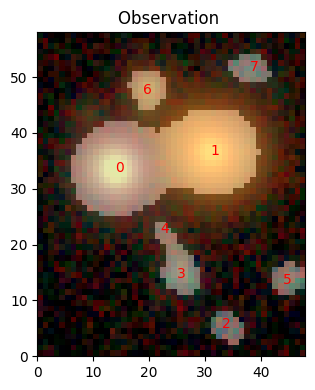
That looks very reasonable. Let’s have a closer look at one of the footprints:

print(footprints[0])

HierarchicalFootprint(
  peak=Peak(y=33, x=14, flux=1.0009099245071411),
  bbox=Box(shape=(31, 30), origin=(18, 0)),
  footprint=bool[31,30](numpy),
  scale=3,
  children=[]
)

Each footprint contains the binary array footprint that indicates the pixels above the detection threshold, a bounding box bbox to place that array in the original image, the primary peak, the scale it was detected on, and, possibly, children.

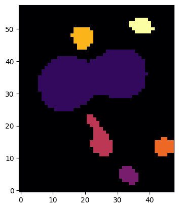
But there are no children here, even though it looks like sources 0 and 1 should be in the same footprint on scale 3, so where’s the hierarchy? By default, the hierarchy is flattened and peaks in the same footprints are split into separate sources by a watershed algorithm, which means that we get footprints like this:

im_shape = obs.frame.bbox.shape[1:]
footprint_map = jnp.zeros(im_shape)
for i,fp in enumerate(footprints):
    footprint_map += sc2.bbox.insert_into(
        jnp.zeros(im_shape),
        (i+1)*fp.footprint,
        fp.bbox
    )
plt.imshow(footprint_map)
plt.show()

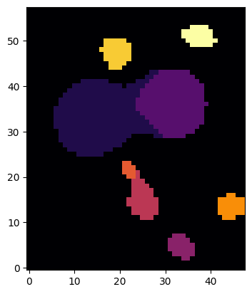
Having non-overlapping footprints is reasonable for un- or weakly resolved sources, like most sources in this observation. If we want to fully acknowledge the possible overlap between sources, we can prevent the flattening and peak splitting:

footprints = sc2.detect.hierarchical_footprints(
    obs,
    scales=scales,
    K=K,
    min_area=min_area,
    split_peaks=False,
    flatten=False,
)
print(footprints[0])

footprint_map = jnp.zeros(im_shape)
for i,fp in enumerate(footprints):
    footprint_map += sc2.bbox.insert_into(
        jnp.zeros(im_shape),
        (i+1)*fp.footprint,
        fp.bbox
    )
plt.imshow(footprint_map)
plt.show()

HierarchicalFootprint(
  peak=Peak(y=33, x=14, flux=1.0009099245071411),
  bbox=Box(shape=(37, 40), origin=(15, 0)),
  footprint=bool[37,40](numpy),
  scale=3,
  children=[
    HierarchicalFootprint(
      peak=Peak(y=36, x=31, flux=0.5996347665786743),
      bbox=Box(shape=(15, 16), origin=(29, 24)),
      footprint=Footprint(
        footprint=bool[15,16](numpy),
        peaks=[Peak(y=36, x=31, flux=0.5996347665786743)],
        bounds=((29, 44), (24, 40))
      ),
      scale=3,
      children=[]
    )
  ]
)

Source 0 now contains what we used to call source 1 as its child, and its footprint covers both. The same happens with the smaller sources 2 and 4.

So, we now have a list (either hierarchical or flattened) of detected sources with their peaks and outlines from a multi-scale filtering method.

Hierarchical Initialization

Finding good guesses for sources in crowded or blended scenes is hard. But the hierarchical footprints allow us to go back and extract sources from the observation. The method scarlet.init.hierarchical_sources() performs the same starlet filtering and hierarchical detection as shown above, and then goes through all scales (from the largest to the smallest) and removes the contributions of each source within its footprint.

model_frame = sc2.Frame.from_observations(obs)

with sc2.Scene(model_frame) as scene:
    infos = sc2.init.hierarchical_sources(
        obs,
        scales=scales,
        strict=strict,
        K=K,
        min_area=min_area
    )
    for sinfo in infos:
        sc2.Source(sinfo.center, sinfo.spectrum, sinfo.morphology)

Let’s check what we have in scene:

sc2.plot.scene(
    scene,
    obs,
    norm=norm,
    show_model=True,
    show_rendered=True,
    show_observed=True,
    add_boxes=True,
);

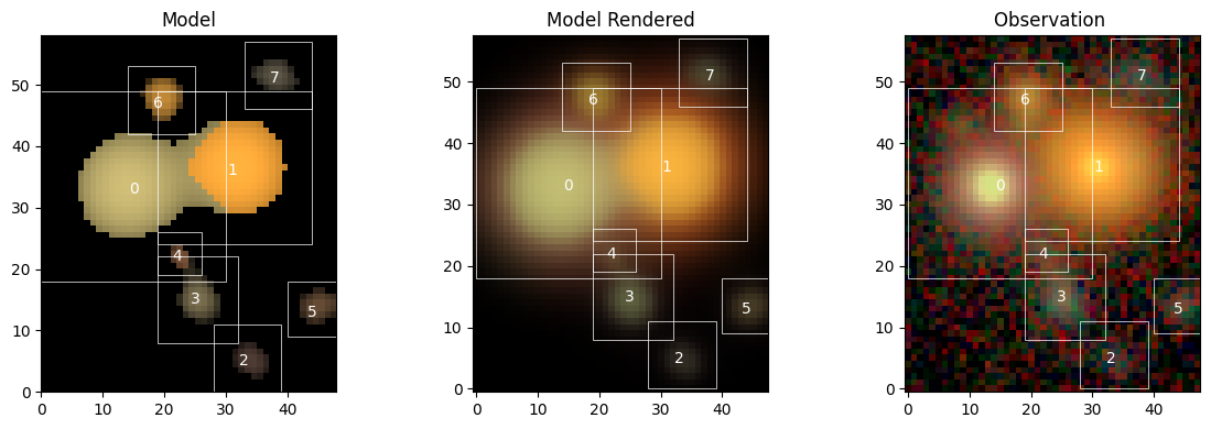
Not too bad…

Initialization with Given Catalog

Often we already have a detection catalog from some previous processing stage (in fact, we have one for this HSC example). So, scarlet2.detect.hierarchical_footprints() and scarlet.init.hierarchical_sources() accept an argument catalog with RA/DEC coordinates. When provided, the methods will go through the catalog list and report only footprints/sources at those locations, or None. Let’s demonstrate:

with sc2.Scene(model_frame) as scene:
    infos = sc2.init.hierarchical_sources(
        obs,
        scales=scales,
        strict=strict,
        K=K,
        min_area=min_area,
        catalog=catalog
    )
    for sinfo in infos:
        sc2.Source(sinfo.center, sinfo.spectrum, sinfo.morphology)

sc2.plot.scene(
    scene,
    obs,
    norm=norm,
    show_model=True,
    show_rendered=True,
    show_observed=True,
    add_boxes=True,
);

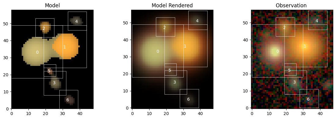
You can see that the order of some sources has changed, and that what used to be called “source 5” on the right edge of the image is not initialized because it is not in the provided detection catalog. But we can now proceed with fitting the scene.